Goal: Collision-free motion generation in unknown environments for robotic manipulation.

MπNets: e2e neural model to generate collision-free, smooth motion from just a single depth camera observation
Trained on 3+ million motion planning problems in 500,000 environments
- Only in simulation
MπNets transfer well to real robot with noisy partial point clouds

Code available at https://github.com/NVlabs/motion-policy-networks

Global planning

"Global" - planner requires prior knowledge (map, complete model) of the entire environment (e.g., all obstacles) from the robot's starting position to its final goal.

🔖 3 camps of global planning:
- Search
  - Break down the entire global environment into a rigid, discrete grid, then mathematically search across that grid to find the shortest continuous path from start to finish.
  - Fast, complete, guaranteed optimal
  - Requires construction of a discrete graph, which hinders these algorithms in continuous spaces and for novel problems not well covered by the current graph (not good for dynamic environments).
  - e.g., A*
- Sampling
  - Functions in a continuous state space by drawing samples and building a tree → when the tree has sufficient coverage of the planning problem, the algorithm traverse the tree to produce the final plan
  - Continuous, probabilistically complete, some are asymptotically optimal
  - Under practical time limitations, their random nature can produce erratic (though valid) paths
  - e.g., RRT (randomly drop points [sample] across the entire global space → connect those points to build a tree of safe movements → eventually link the start to the goal)
- Optimization
  - Generates paths with non-linear optimization & can consider multiple objectives - smoothness of the motion, obstacle avoidance, convergence to an end effector pose
  - Not complete, probabilistically complete, asymptotically optimal, ... - none of these in its vanilla form!
  - Requires careful tuning of the cost functions to ensure convergence to a desirable path, & prone to local minima; can also be slow.
🔑 Search and sampling-based planners optimize for path length in the given state space (e.g. configuration space) while avoiding collisions:
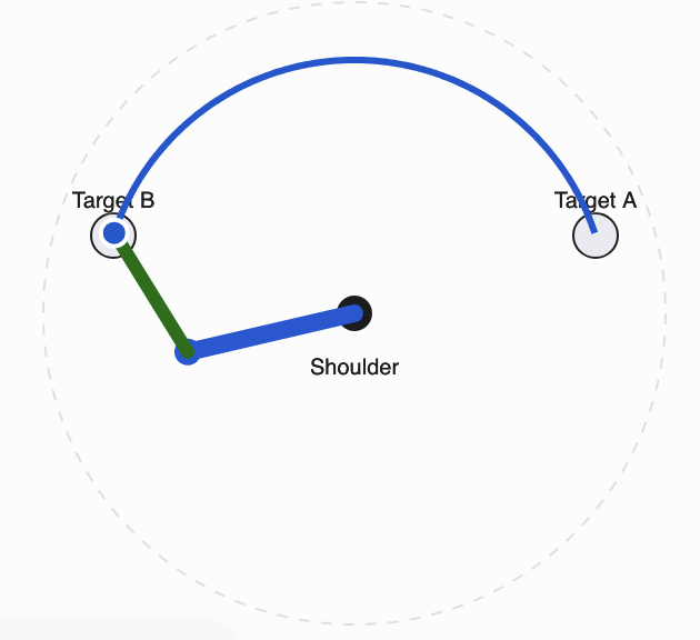
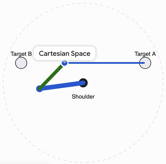
- ⚠️ An optimal path in configuration space is not necessarily optimal for the end-effector in cartesian space - & human motion tends to minimize hand distance traveled, so what appears optimal for the algorithm may be unintuitive for a human/operator
  - Usually, search and sampling planners live in C-space (joint space) but the robot operates in task space (3D world) → an optimal path in C-space = shortest distance between the starting joint angles and the ending joint angles, but because the robot arm is made of rotating links, a small angle changes in joint space can cause the hand to swing in a wide, sweeping arc in Cartesian space → yikes!
    - Joint space optimal path:
    - Cartesian space optimal path:
  - ❓ Why do planners live in C-space? Why can't a planner live in Cartesian space and then have an IK solver handle the rest?
    - In C-space, every point $q$ uniquely and completely defines the exact position of every motor, link, and cable on the robot - if $q$ is marked as "collision-free," the entire robot is safe!
    - In Cartesian space, a 6D pose $p$ $p$ only defines the end-effector - it tells us nothing about where the elbow is → cannot check a Cartesian point for collisions because it doesn't specify the state of the robot's geometry
      - So if we plan a nice straight collision-free line for the gripper in Cartesian space, the robot's elbow might be smashing through a table to achieve it.
    - So, C-space search requires only forward kinematics (moving from $q_1$ to $q_2$ is defined through FK), while Cartesian search would require inverse kinematics on every node in the path → way too slow to do at every step in a search algorithm!
    - Also, many robots have more DoF in C-space (e.g., 7dof for iiwa/franka) than Cartesian space (fixed 6dof 3D pose), so if we only plan in Cartesian space, the planner ignores the free DoF's.
- In the manipulation domain, goals are typically represented in end effector task space. How can we get the planner to also minimize distance in the task space as a secondary goal?
  - Motion optimization!

Local control

"Local" - planner reacts to immediately incoming information, and cannot see the global layout.

🔖 TL;DR: the planner is akin to driving with headlights in a dense fog - can ensure collision-free motions + speed + smoothness, but highly local and may fail to find a valid path in complex environments.
Example: artificial potential fields:
- Imagine the robot's EE is a positively charged metal ball.
  - Make the target a negative charge: it exerts an attractive force, constantly pulling the robot toward it.
  - Make every obstacle a positive charge: exerts a repulsive force, pushing the robot away if it gets too close.
- Local controller runs a simple loop:
  1. Calculate the pull of the target
  2. Calculate the push of the nearest obstacles
  3. Add those forces together to get a combined vector
  4. Take a tiny step in the direction of that arrow
  5. Repeat 500 times a second.
- Problem: local controllers can get stuck in situations where (1) and (2) cancel each other out (e.g. when it wanders to the middle of a U-shaped obstacle) - local minimum trap!
^ VLAs (e.g. π0.5) that directly output motor commands based on a camera feed essentially run a learned local controller - operates at high speeds, reacts to the local environment (what the camera sees right now), and prioritizes smooth, immediate actions over long-term, global graph-searching.

Imitation learning

Train a policy from expert demonstrations, with limited knowledge of the expert's internal model.

💡 For motion planning problems, we can use a traditional planner as the expert demonstrator (with perfect model of the scene during training) and learn a policy that removes the need for an explicit scene model at test time
Popular imitation learning methods:
- Inverse RL [read into more!] - assumes expert optimality and learns a cost function accordingly
  - Standard RL: you give the robot a reward function (e.g., +10 for reaching the door, -1 for hitting a wall) and the robot figures out the actions.
  - Inverse RL (IRL): you give the robot the actions (expert demonstrations), and the math works backward to figure out what the reward/cost function must have been.
    - Once IRL extracts this hidden cost/reward function, we can throw away the expert data and use standard RL to train the robot on that new function.
  - 🔑 Core assumption: to reverse-engineer the goal, the algorithm must assume the given demonstrations are acting rationally and optimally. i.e., if the expert is suboptimal and loves doing loops, the reverse-engineering will rationalize that loops are necessary for reaching the door → yikes!
- Behavior cloning (BC) - directly learns the state-action mapping from demonstrations, regardless of the expert's optimality
  - essentially standard supervised learning applied to robotics - give the model a dataset of (state, action) pairs from an expert, the model learns to predict the action given the state
  - 💡 BC, at best, does blind mimicry of the expert data - it does not try to infer intent from the data (which is what IRL does) → the model is a mapping function $f(\text{state}) = \text{action}$ that aims to minimize $\mathcal{L} \sim \text{loss}(f(\text{state}), \text{action})$ .
🔖 MπNets employs BC because producing optimal plans for continuous manipulation problems is hard
⚠️ Challenges in BC: distributional shift and data variance in long-horizon tasks
- Distributional shift: (compounding error problem)
  - Training distribution: During training, the model only sees the states the expert visited - because the expert is good, these states represent a narrow, safe corridor of "safe driving"
  - Inference time distribution shift: during inference, say the model makes a small mistake. Now, the robot is in a state slightly outside the "safe corridor" it saw during training
  - → Because the model has never seen this new, slightly-off state, its next prediction worsens → errors compound exponentially, yikes!
- Data variance: long-horizon tasks take many sequential steps to complete, and the longer the sequence, the more potential variance (number of possible state-chains increases exponentially)
  - Multimodality: in long tasks, there are many valid ways to succeed - an expert might grab the butter with their left hand one day, and their right hand the next. When the BC model sees this during training, it might average (mode averaging) the two actions together - could be no longer valid!
  - Long tail of edge cases: longer tasks = more likely to encounter rare situations → because these edge cases rarely occur in the expert demonstration data, the model has high variance in these states - it hasn't seen enough data to learn the pattern.
- Techniques to address these challenges:
  - Randomization, noise injection, regret optimization, expert correction, ...

Summary of MπNets goal, relative to prior related works

Use BC to learn an e2e motion planner
- Subside some deficits of BC by designing a learnable expert, increasing scale + variation of the data, and using a sufficiently expressive policy model
- e2e - unlike Motion Planning Nets, MπNets throws the entire scaffolding of a standard planning system out the window (instead of learning something that makes search faster in a standard planning system, they want to replace the entire planning system with a learned model)

Learning motion planning - MπNet setup!

Problem formulation

Inputs

Robot configuration $q_t$ $q_{t}$
- Normalized s.t. each element $\in [-1, 1]$ , according to the limits for the corresponding joint → $q_t^{||\cdot||}$
Segmented, calibrated point cloud $x_t$ $x_{t}$
- Calibrated in the robot's base frame
- Encodes 3 segmentation classes: (raw point cloud from a depth camera = massive list of 3D coordinates $(x,y,z)$ $(x, y, z)$ , to inform the NN what each dot represents, MπNets segments the point cloud - adds a class label to every single point in the cloud, s.t. $(x, y,z) \mapsto (x, y, z, c)$ $(x, y, z) \mapsto (x, y, z, c)$ where $c$ $c$ is the class)
  1. the robot's current geometry
  2. scene geometry
  3. target pose
- Targets are inserted into the point cloud via points sampled from the mesh of a floating end-effector placed at the target pose.
  - 💡 How do we tell the NN where to go? → because the MπNets model only accepts init robot config + point clouds as input, the point cloud needs to embed the target robot EE pose → they do this by adding the target pose as a class to the point cloud
- Example:
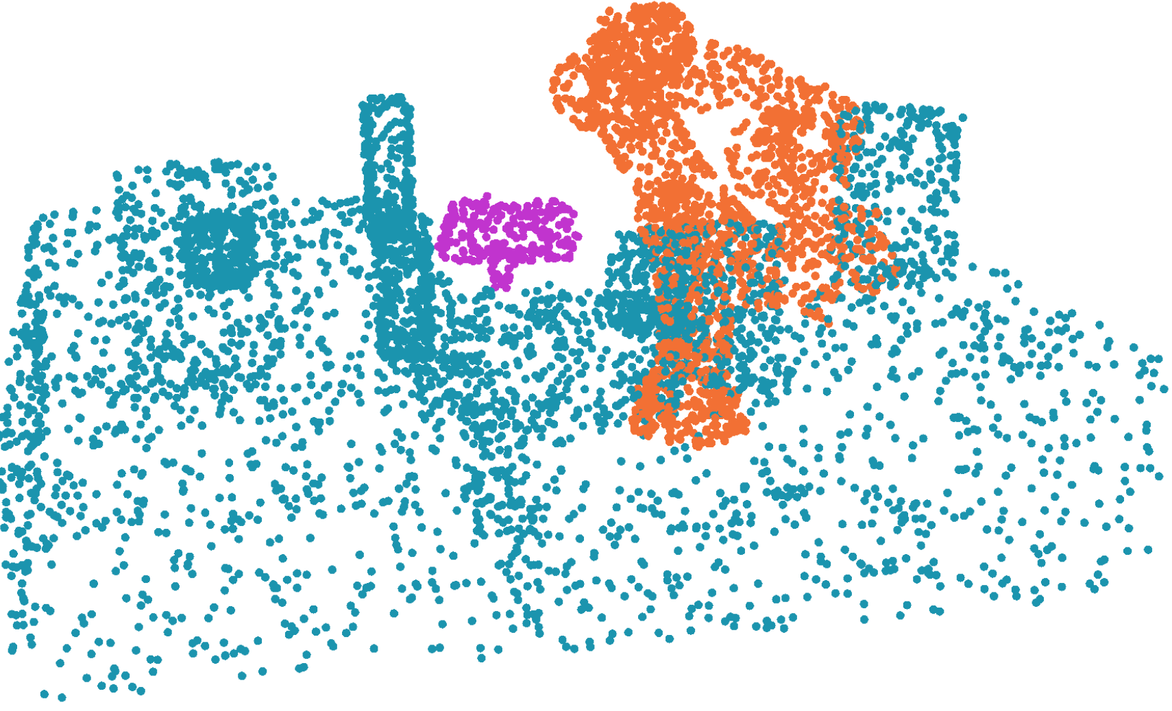
  - ^ 3 point cloud segmentation classes in different colors (orange, cyan, magenta)

Outputs

The network produces a displacement within normalized configuration space $\dot{q}_t^{||\cdot||}$ : to get to the next predicted state $\hat{q}_{t+1}$ , we do: $\hat{q}_{t+1} = \text{unnormalize} \left[\text{clamp\_between\_[-1,1]}\left(q_t^{||\cdot||} + \dot{q}_t^{||\cdot||}\right)\right]$ During training, we use $\hat{q}_{t+1}$ to compute the loss (compare it to the expert's $q_{t+1}$ ), and when executing, we use $\hat{q}_{t+1}$ as the next position target for the robot's low-level controller.

Model architecture

MπNets is a spatial and temporal autoregressive model!

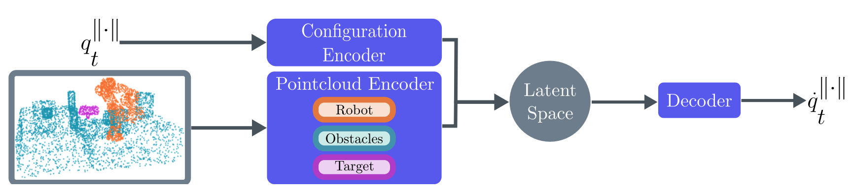
2 encoders: one for the point cloud & one for the robot's current configuration
1. Point cloud encoder: PointNet++ architecture (learns a hierarchical point cloud representation + encodes a point cloud's 3D geometry)
2. Robot configuration encoder: fully connected MLP
1 decoder: fully connected MLP
Total 19M params
🔖 Architecture details in Appendix C.
❓ If the point-cloud is robo-centric, how do we get the robot to be in the point cloud? Does robo-centric mean the point-cloud is constructed from a camera at the robot base? But then how would the robot be imaged by this camera? Or do we have external cameras that we use to construct a point cloud of the full scene (including the robot), and then transform the point cloud s.t. the robot base is at $(0,0,0)$ $(0, 0, 0)$ ?
- [According to Gemini, not verified yet] Pipeline of how a robot-centric point cloud is actually constructed:
1. Capture the scene, ignoring the robot
  - using cameras throughout the room / mounted on the robot
  - generate point cloud
2. Forward kinematics
  - the robot doesn't need to look at itself to know where its body is - we can take joint state $q$ , use FK + robot's URDF to get the exact mesh of where the robot is in 3D space
3. Inject the virtual robot
  - uniformly sample points across the surface of the CAD meshes from step (2) → drop them into the camera's point cloud from step (1)
4. Transform to the base frame
  - transform the entire unified point cloud s.t. the origin point $(0, 0, 0)$ sits at the physical base of the robot

Loss function

The network is trained with a compound loss function := a BC loss to enforce accurate predictions + a collision loss to safeguard against catastrophic behavior.

Geometric loss for BC

To encourage alignment between the prediction $\hat{\Delta}q_t$ and the expert $q_t$ , compute a geometric loss across a set of 1,024 fixed points ( $i$ ) along the surface of the robot: $\mathcal{L}_\text{BC} (\hat{\Delta}q_t) = \sum_i \big|\big|\hat{x}^i_{t+1} - x_{t+1}^i\big|\big|_2 + \big|\big|\hat{x}^i_{t+1} - x_{t+1}^i\big|\big|_1$ $\hat{x}^i_{t+1} = \phi^i(q_t + \hat{\Delta}q_t)$ and ${x}^i_{t+1} = \phi^i(q_t)$ , where $\phi^i(\cdot)$ represents a forward kinematics mapping from the joint angles of the robot to point $i$ defined on the robot's surface ( $\phi^i$ takes the current joint angles $q_t$ and outputs the 3D Cartesian coordinate $(x,y,z)$ of the $i$ th dot).

💡 Loss = sum of the L1 and L2 distances between corresponding points on the expert and the prediction after applying the predicted displacement
- 🔑 L1 and L2 both used - so that we penalize large and small deviations $||\hat{x}-x||_1 = |\hat{x}_1 - x_1| + |\hat{y}_1 - y_1| + |\hat{z}_1 - z_1|, ||\hat{x} - x||_2 = \sqrt{(\hat{x}_1 - x_1)^2 + (\hat{y}_1 - y_1)^2 + (\hat{z}_1 - z_1)^2}$
- L2 norm handles massive mistakes - a point that is 10 inches off target generates a massive loss penalty (100), producing a huge gradient that violently yanks the NN's prediction back toward the expert trajectory.
  - ⚠️ However, as the error gets very small (e.g. 0.1 inches), the gradient effectively vanishes, and the NN stops trying to improve
- L1 norm provides a steady, constant pressure forcing the network to keep adjusting until the error is exactly 0
💡 Loss is in task-space and not in C-space to ensure task-space consistency: if we calculate loss in C-space (compare joint angles directly: $q_t - (q_{t-1} + \hat{\Delta}q_t)$ $q_{t} - (q_{t - 1} + \hat{Δ} q_{t})$ ), the math treats a 2˚ error at the robot's shoulder exactly the same as a 2˚ error at its wrist → but in task-space, a 2˚ error at the wrist might move the hand by 1mm while a 2˚ error at the shoulder might swing the hand 10 inches.
- By having the loss in task-space, the geometric loss corresponds to actual physical deviation in the real world.

Note on the autoregressive training setup

In BC, we use a technique called teacher forcing:

During training: $\hat{q}_{t+1} = q_t^{(\text{expert})} + \hat{\Delta}q_t \text{ where } \hat{\Delta}q_t = \text{model}\left(q_{t}^{\text{(expert)}}, x_{t}^{\text{(expert)}}\right)$ where $x_t$ is the point cloud observation at that exact moment.
During inference: $\hat{q}_{t+1} = \hat{q}_t^{(\text{prediction})} + \hat{\Delta}q_t \text{ where } \hat{\Delta}q_t = \text{model}\left(q_{t}^{\text{(prediction)}}, x_t^{\text{(actual)}}\right)$

Collision loss

Hinge-loss "inspired by motion optimization": $\mathcal{L}_{\text{collision}} = \sum_i \sum_j \big|\big|h_j(\hat{x}^i_{t+1})\big|\big|_2, \quad h_j(\hat{x}^i_{t+1}) = \cases{D_j (\hat{x}_{t+1}^i), & if D_j(\hat{x}_{t+1}^i) \leq 0 \\ 0, & if D_j(\hat{x}_{t+1}^i) > 0 }$ where $D_j$ are the signed distance functions of all the obstacles in each scene; i.e. SDF = $\{D_j(\cdot)\}_j$ .

For a given closed surface, its SDF maps a point in Euclidean space to the minimum distance from the point to the surface.
If the point is inside the surface (aka. collision!), the function returns a negative value.
💡 $\mathcal{L}_\text{collision}$ $L_{collision}$ penalizes all surface points $i$ $i$ on the robot that have negative/0 distance to any obstacle surface
- "distance between robot point $i$ to obstacle surface" in SDF = "distance between robot point $i$ to closest point on obstacle surface"

Why is this called a "hinge-loss" and how is it inspired by motion optimization?

$\mathcal{L}_\text{collision}$ is called a "hinge-loss" because its graph is completely flat (0) on one side of a threshold, then slopes up on the other side, creating a sharp "hinge" corner at the threshold.
It is "inspired by motion optimization" in the sense that unlike BC which only cares about imitation (no concept of the actual physical space), motion optimization algorithms takes a mathematical path and physically push it out of obstacles by calculating the SDF
💡 Combined, $\mathcal{L}_{\text{BC}}$ and $\mathcal{L}_\text{collision}$ enforce both blind data mimicry and true physical geometry

Training implementation details

MπNets is trained for single-step prediction, but during inference, it is recursively used to create closed-loop rollouts, i.e. during inference:

$\hat{q}_{t+1}^{(\text{prediction})} = \hat{q}_t^{(\text{prediction})} + \hat{\Delta}q_t \text{ where } \hat{\Delta}q_t = \text{model}\left(q_{t}^{\text{(prediction)}}, x_t^{\text{(actual)}}\right)$

⚠️ ^ this leads to compounded noise in subsequent inputs (as $t$ $t$ increases, $\hat{q}_t$ $\overset{q}{^}_{t}$ gets increasingly noisy because it folds in all the noise from prior predictions) → covariate shift
- MπNets attempt to resolve this covariate shift (aka. "increase robustness") using 2 methods:
  1. Apply Gaussian noise to the joint angles of each input configuration, which in turn affects the corresponding points in the point cloud, apssed as input to the network
  2. For each training example, they generate a unique point cloud during training (i.e., during each epoch, the network sees 163.5M unique point clouds)
    - ❓ "unique point cloud" - what changes between point clouds of the same scene each epoch?
      - Random sampling: to get the point cloud, the system randomly samples points from the surfaces of the 3D objects in the simulation - so by regenerating a point cloud of the same scene each epoch, epoch 1 might have 500 points that fall on the left side of a coffee mug, while epoch 2 might have 500 points that fall slightly more on the right side of the mug
      - Gaussian noise: robot config will slightly differ due to method (1)
- The network is trained with a single set of weights across the entire dataset

Closed-loop vs. open-loop

Closed-loop: the "loop" is closed between acting and perceiving
- e.g., the robot takes an action, checks its sensors (vision, joint encoders) to see exactly what happened, and then calculates the next action based on that new reality
Open-loop: the "loop" is open between acting and perceiving
- e.g., generating an entire trajectory all at once (standard A*) and handing it to the motors to execute blindly

Covariate shift

What is the relationship between "covariate shift" in ML and "covariates" in statistics?

ML: In ML, "covariates" are the input variables you feed into a model.
- "Covariate shift during inference" means the type of data you are feeding the model during inference no longer matches the type of data it saw during training.
Statistics: In stats, when you are trying to find a cause-and-effect relationship, there are 2 main types of variables:
- Dependent variable $Y$ : the thing you are trying to predict (e.g., a person's risk of heart disease)
- Independent variable $X$ : the factors you think are causing or predicting $Y$ (e.g., age, weight, smoking habits)
- The independent $X$ variables are called "covariates" because they co-vary (change alongside) the outcome you are studying
🔑 ^ ML and stats link in the sense that:
- Dependent variable $Y$ = network's output/label (in MπNet, this is $\hat{\Delta}q_t$ )
- Covariates $X$ = input features fed into the network (in MπNet, this is the 3D point cloud and the current joint angles $q_t$ )

Procedural data generation

MπNets is trained with a dataset consisting of solutions to 3.27M unique planning problems across 575,000 unique, procedurally generated environments.

Procedural data generation: creating training data automatically using an algorithm ("procedures") rather than having a human manually build it.

Large-scale motion planning problems

Each planning problem is defined by 3 components:

Scene geometry
Start configuration
Goal pose

🔑 Dataset consists of randomly generated problems across all 3 components ^
🔖 3 classes of problems of increasing difficulty: cluttered tabletop with (1) randomly placed objects, (2) cubbies, and (3) dressers

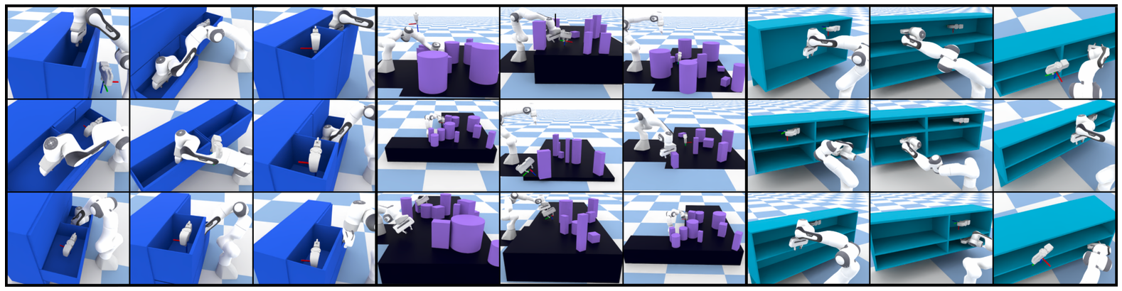
MπNets procedural data generation problem types.png

Procedural generation steps:
1. Build scene environments
2. Generate robot configurations (generate a set of potential end-effector targets and the corresponding IK solutions)
3. Randomly choose pairs of these configurations (step 2) and verify if a plan exists between them using the expert pipeline (details in Sec. 4.2 + Appendix D)

Expert pipeline

🔖 Expert pipeline is designed to produce high quality demonstrations we want to mimic - i.e. trajectories with smooth, consistent motion & short path lengths.
- "consistency" - quality and repeatability of an expert planner (Appendix B)
2 candidates for the expert:
1. Global planner - typical SOTA C-space planning pipeline
2. Hybrid planner - they engineered this specifically to generate consistent motion in task-space
For both planners ^: reject any trajectories that produce collisions, exceed the joint limits, exhibit erratic behavior (i.e. high jerk), or have divergent motion (i.e. final task space pose is more than 5cm from the target)

Global planner

Consists of off-the-shelf components of a standard motion planning pipeline:

IK
C-space AIT* (Adaptively Informed Trees - asymptotically optimal path-planning algorithm)
Spline-based, collision-aware trajectory smoothing

Generated 6.54M trajectories across 773K environments.

❓ But didn't they say they trained on 575K environments earlier?
- Yes, but it appears that the full dataset has at least 773K environments - so around 200K are held out as eval datasets
- 6.54M trajectories - earlier, it says that the dataset had 3.27M planning problems → 3.27 * 2 = 6.54 → a planning problem is defined as finding a path from point A to point B. Assuming that a robot's physical environment doesn't change while it is moving, any safe, collision-free path from A to B is also a safe+collision free path if you run it backward from B to A.

Hybrid planner

The hybrid planner ("hybrid" because it combines a global planner with a local controller) is designed to produce consistent motion in task space.

("hybrid" because it combines a global planner with a local controller)
Global planner: AIT*
- looks at the whole scene and drops a series of waypoints through the physical Cartesian space, guaranteeing a path that avoids local-minima paths
Local controller: Geometric Fabrics (https://arxiv.org/abs/2109.10443)
- the system feeds the waypoints obtained from the global planner to the local controller, which smoothly fills in the paths between waypoints to create the full trajectory
- Geometric Fabrics - uses differential geometry to bend the mathematical space the robot operates in → defines the environment as a set of overlapping, warped energy landscapes s.t. the robot just "rolls" downhill toward the target, naturally flowing smoothly around obstacles

AIT* produces an efficient EE path & Geometric Fabrics produce geometrically consistent motion.

⚠️ As the robot moves through the global planner waypoints, its speed can vary - they fit a spline to the path + retime it to have steady velocity throughout the trajectory
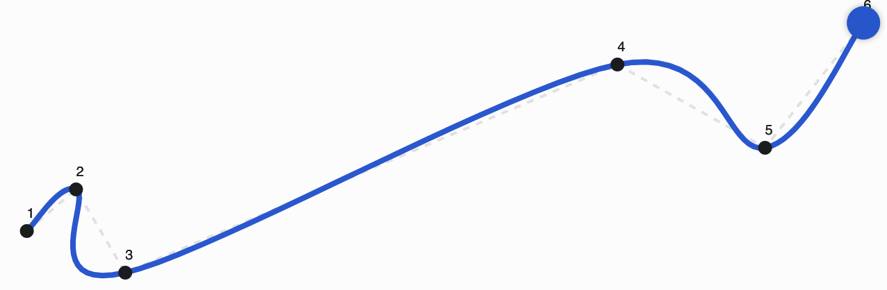
- "spline" := mathematical function that we can bend s.t. it passes through all the waypoints → converts the jagged connect-the-dots path into one continuous, smooth curve
💡 They use hindsight goal revision for the hybrid planner! (see later section of notes)

Discrete collision checking

A discrete collision checker breaks the continuous motion trajectory down into a series of waypoints ("snapshots") - at each snapshot, the algorithm runs to check if the robot's 3D mesh is intersecting with an obstacle's 3D mesh.

⚠️ Discrete collision checkers can miss collisions due to the physics problem known as tunneling - if the distance between the snapshots is larger than the thickness of an obstacle, the robot can effectively teleport through it - yikes!

Hindsight goal revision (HGR)

TL;DR: move the goalposts after the robot has already shot!

⚠️ Problem: Geometric Fabrics often fail to converge to a target - i.e., say the original problem (defined during data generation) is to get from point A to B. Geometric Fabrics often will end up at a spot B' that is 2 inches short of B.
- If this trajectory outputted by Geometric Fabrics that slightly misses the target pose B is put into a behavior cloning dataset, the network would see a target coordinate + expert demonstrations that stop 2 inches away from the target - the model would learn to miss targets :"(
- 🔑 Solution: HGR! Instead of throwing out the trajectory produced by Geometric Fabrics, they take the exact XYZ coordinate where the robot's hand actually stopped in this trajectory (B') and overwrite the original target coordinate in the dataset with B', i.e. set $B = B'$ .
- ^ by retroactively moving the finish line to exactly where the robot parked, every trajectory generated becomes a "perfect" demonstration of the robot successfully reaching a goal - so the network learns that success := arriving exactly at the provided target coordinates.
❓ Why is HGR valid to do?
- Because the network only needs to train on the physics of the trajectory - learning to get from A to B is equivalent to learning to get from A to B', because the goal is for the network to learn the mechanics of getting from start poses to end poses.
- So HGR is equivalent to changing the label on the data from [a failed attempt to reach B] to [a perfect attempt to reach B']
- ^ increases data efficiency!

Experimental evaluation

Separate test set with new problems (unique randomly generated environment + target + start configuration)
3 test sets: each has 1800 problems with 600 in each of the three types of envs
1. problems solvable by global planner
2. problems solvable by hybrid planner
3. problems solvable by both

Quantitative metrics

Each policy is rolled out until it matches one of two termination conditions:

Euclidean distance to the target is within 1cm
Trajectory has been executed for 20s

Metrics:

Success rate - trajectory is successful iff final position + orientation target errors are below 1cm and 15˚, & no physical violations
Time - wall time for each successful trajectory
- also measure Cold Start Time - average time to react to a new planning problem
Rollout target error - L2 position + orientation error between the target and final end-effector pose in the trajectory
Collision rate - rate of fatal collisions (self + scene collisions)
Smoothness - use spectral arc length (SPARC) & consider a path "smooth" if its SPARC values in joint and EE space are below -1.6

Comparison to methods with complete state

Most methods to generate motion in the literature assume access to complete state information in order to perform collision checks - in the comparisons in this section, all baseline methods are provided with an oracle collision checker

^ for MπNets, providing oracle collision checker := providing a point cloud sampled uniformly from the surface of the entire scene
🔑 Takeaways:
- MπNets trained with data from the hybrid expert outperformed the hybrid expert on the global planner-solvable test set!
  - likely due to:
    - reject sampling to reduce erratic + divergent behavior in the training dataset
    - HGR to turn an imperfect hybrid expert into a perfect one for the model to train on
- MPNets vs. MπNets:
  - MPNets input = start, goal, flattened representation of the obstacle points; output = sample
    - guarantees completeness by using a traditional planner as a fallback if the neural planner fails
    - e.g., classical planner RRT* obtains a traj by playing a massive game of connect-the-dots:
      1. Randomly generate a sample $q$ (random joint angles) [this is where MPNets samples get inserted]
      2. Check if $\text{FK(q)}$ causes the robot to hit a wall
      3. If it is safe, drop a dot at $q$ and try to draw a line connecting it to the previous dots (checks for collisions across this connecting line using discrete collision checker)
      4. Repeat until the dots accidentally connect the start pose to the goal pose
  - MPNets is more data efficient (utilizes a trad planning system so it is effective with a small dataset / on OOD problems), but does not scale to more complex scenes even with more data
- Local task-space controllers:
  - STORM and Geometric Fabrics make local decisions that can lead them to diverge from the target in complex scenarios (i.e. cluttered environments / those with pockets)
    - ^ prior environment knowledge + expert tuning can lead to good results, but these parameter values do not generalize
  - MπNets is also a local policy! But it encodes long-term planning info across a wide variety of envs from training, which makes it less prone to local minima (especially in unseen envs)
  - MπNets target convergence rate is higher than STORM/Geometric Fabrics but collision rate is worse than either local controller
  - MπNets performance deteriorates on OOD problems - could be improved with:
    - more robust expert
    - finetuning
    - DAgger
- Choice of expert pipeline affects the performance of MπNets!
  - 🔑 MπNets-H (trained only on data from hybrid expert) does best across target convergence + collision avoidance
  - Authors hypothesize that an expert with the consistency of the hybrid planner and the generality of the global planner would further improve MπNets performance
    - Consistency - an expert is consistent if, when given the exact same problem, it will solve it the exact same way every single time, with smooth predictable motions.
      - RRT*, AIT* are inconsistent because they rely on random sampling to find paths - if you ask a global planner to go around a coffee mug, it might go left this time, right next time, over the top nextx2 time, ...
      - Geometric Fabrics is consistent because the mathematical downhill landscape is fixed, and a ball rolled down the same landscape will always behave largely similarly
      - 🔑 Neural networks like consistency because it makes it easy to memorize the correct behavior
    - Generality - generality is the ability of an algorithm to successfully solve any valid puzzle thrown at it
      - Global planners are very general - it searches the entire room, backtracks when it gets stuck, ... - will eventually solve any solvable maze
      - Hybrid planners/local controllers are less general, because local controllers risk getting permanently trapped in local minima - not guaranteed to solve any solvable maze

Comparison to methods with partial observations

Partial observation setup - a single-view depth camera setting in simulation

🔑 MπNets success rate only suffers a minor drop, collision rate increases from <1% to 3% due to occlusions
To setup global planner's environment as "partial observation" - used a voxel-based reconstruction → a voxel is filled only if a 3D point is registered within it
- Global planner plans on top of this voxel representation
Conclusion: Global planner suffers from 5x more collisions than MπNets in partial observation setup

Ablations

Takeaways:

MπNets scales with more data - saturates at 1.1M trajectories
- 1 data point := (point_cloud, joint_state, target_displacement) (target_displacement = an array of dim_q representing the tiny delta between the robot's current joint angles and the joint angles it should have in the next frame, according to the expert planner) → each trajectory generates many data points, depending on how finely we slice the trajectory into time frames!
Robot point representation improves performance - inserting the robot point cloud at the specific configuration improves success rate from 65.06% (point cloud doesn't contain robot) to 95.33% (point cloud contains robot) [robot config q vector is always fed to the model]
- 💡 For us - could explore if adding target to point cloud helps (point cloud with EE in target pose vs. point cloud without EE in target pose)
HGR improves target convergence of model
Noise injection improves robustness - training without injecting noise into input $q_t$ decrease policy performance by 10.72%

Dynamic environments

MπNets still works if the environment is continually changing, as long as the changes are not fast!

💡 By construction, MπNets implicitly approximates dynamic motion as a sequence of static motions (it predicts $\Delta q_t$ $Δ q_{t}$ given $q_t$ $q_{t}$ , assuming that the world is constant between $t$ $t$ and $t+1$ $t + 1$ ).
- So if the environment moves slow enough s.t. the snapshot between time $t$ and $t+1$ is largely the same, MπNets is reactive enough - otherwise, MπNets will return a $\Delta q_t$ that plans for a $t+1$ world that looks similar to the $t$ world but diverges from the true $t+1$ world (because something in the environment is changing significantly within $[t, t+1]$ time frame)

Real robot eval

MπNets can achieve sim2real transfer on noisy real-world point clouds! Deployed on 7-DOF Franka Emika Panda robot with an extrinsically calibrated Intel Realsense L515 RGB-D camera.

🔖 Depth measurements belonging to the robot are removed and re-inserted using a 3D model of the robot before inference with Mπnets.
- i.e., delete depth measurements corresponding to robot in the point cloud, then use FK + robot's 3D CAD model + known robot $q$ to drop the exact robot point cloud into the full scene point cloud
Demonstrations on real robot are open-loop in static environments (robot takes a single 3D picture at the beginning, calculates the entire sequence of $\Delta q_t$ steps from start to finish, and then executes them blindly) & closed-loop in dynamic environments (robot takes a photo, executes a step, takes a new photo, executes next step, ...)

Camera calibration

Intrinsic params: these describe the internal hardware of the camera - focal length, FOV, ...
Extrinsic params: these describe the exact pose of the camera relative to the world

Limitations

MπNets limitations:

Limited by quality of the expert supervisor
Struggles to generalize to OOD settings
Future directions:
- DAgger
- Domain adaptation
- Combine with ground-truth or learned collision checker (e.g. SceneCollisionNet)

My key takeaways

MπNets is a learned neural local policy: local because it outputs $\Delta q_t$
HGR? Can we do this too?
- Our version of this would be to generate $(b, q, h)$ pairs, run collision-aware IK on $h$ to generate $(b', q')$ that FK's to $\text{FK}(b', q') = h' \approx h$ , and then rewrite the dataset to $(b', q', h')$ so that the FK relationship is exact.
- ^ I guess we don't need to do this though? We could just do: generate $(b, q)$ , check collision, keep $(b, q, h)$ if no collision.
- Conclusion: I don't think we need HGR for our use case.
Robot point representation improves performance - inserting the robot point cloud at the specific configuration improves success rate from 65.06% (point cloud doesn't contain robot) to 95.33% (point cloud contains robot) [robot config q vector is always fed to the model]
- 💡 For us - could explore if adding target to point cloud helps (point cloud with EE in target pose vs. point cloud without EE in target pose)
Look into DAgger + domain adaptation
💡 Could a new way to generate trajectories be to sample EE waypoints and then run smart IK?
- This would be potentially feasible if smart IK could be conditioned on a context window of prior / future poses (so that it could learn "smooth" motions for the joints/links between waypoints) + collision avoidance