Classifier-Free Guidance (CFG)

Problem: How can we control the generated samples? e.g., for a diffusion-based image model, how can we generate only dogs? → need conditional control!

TODOs to clean up notes

• Clarify notation (what is $\tilde{\mu}$, $\epsilon^*$, ...)

Diffusion review

1. Forward process (noise): $$x_0 \sim \text{dataset}\rightarrow \cdots \rightarrow x_{t-1} \xrightarrow{q(x_t \mid x_{t-1})} x_t \rightarrow \cdots \rightarrow x_T \sim \mathcal{N}(0, I)$$
   • The forward noising process is fixed and known: $q(x_t \mid x_{t-1})$
2. Reverse process (denoise):
   • 💡 The true reverse noising process is what we want: $q(x_{t-1} \mid x_t)$, because then we could generate new samples $x_0^*$ by iteratively denoising from samples $x^*_T \sim \mathcal{N}(0, I)$. So we learn a model $p_\theta(x_{t-1} \mid x_t)$ that ideally matches the true reverse process $q(x_{t-1} \mid x_t)$ as closely as possible. $$x_T^* \sim \mathcal{N}(0, I) \rightarrow \cdots \rightarrow x_t^* \xrightarrow{p_\theta(x_{t-1} \mid x_t)} x_{t-1}^* \rightarrow \cdots \rightarrow x_0^* \sim \text{dataset (new sample)}$$

Score function perspective of the diffusion reverse process

Predicting the noise added to an image is mathematically identical to estimating the gradient of the log-probability density of the data (known as the score).

• ^ Let's prove this!

0. Reparameterization trick

The reparameterization trick allows us to rewrite a random variable sampling operation ($x \sim p(x)$) as a deterministic operation combined with an independent, standard noise source.

• 💡 $z \sim \mathcal{N}(\mu, \sigma^2)$ can be equivalently expressed as $z = \mu + \sigma \epsilon$, where $\epsilon \sim \mathcal{N}(0, I)$
• The "reparameterization trick" is broader than just applying to Gaussian distributions - the above statement is just the instantiation applicable to these notes on diffusion models. See Wikipedia for details.

I. Forward process (adding noise)

Let $x_0 \sim q(x_0)$ be a sample from our true data distribution.

• The forward process adds Gaussian noise in $T$ discrete timesteps according to a variance schedule $\beta_1, \beta_2, \ldots, \beta_T$. The transition probability for a single step is: $$q(x_t \mid x_{t-1}) = \mathcal{N}(x_t; \sqrt{1- \beta_t}x_{t-1}, \beta_t I)$$
  • 📍 $\mu_t = \sqrt{1 - \beta_t} x_{t-1}$ is defined with the multiplier $\sqrt{1 - \beta_t}$ to keep the variance of each noising step at a constant (1). Assuming the original data $x_0$ has been normalized so that its variance is roughly $I$ (identity matrix, meaning variance of 1 for each pixel¹), let's examine the variance of $x_t$: $$\text{Var}(x_t) = \text{Var}\left(\sqrt{1 - \beta_t}x_{t-1} + \sqrt{\beta_t} \epsilon_{t-1}\right), \quad \epsilon_{t-1} \sim \mathcal{N}(0, I) \quad \text{(reparameterization trick)}$$ Because $x_{t-1}$ and $\epsilon_{t-1}$ are independent, the variance of their sum is the sum of their variances. Since $\text{Var}(cX) = c^2 \text{Var}(X)$: $$\text{Var}(x_t) = (\sqrt{1 - \beta_t})^2 \text{Var}(x_{t-1}) + (\sqrt{\beta_t})^2 \text{Var}(\epsilon_{t-1}) = (1 - \beta_t)\text{Var}(x_{t-1}) + \beta_t(I) = 1$$As shown, by scaling the mean by $\sqrt{1 - \beta_t}$, we ensure that the total variance remains stable (near $I$) throughout the entire forward process (ultimately, we want $x_T \sim \mathcal{N}(0, I)$).
• When we have two independent Gaussian variables $X \sim \mathcal{N}(\mu_X, \sigma^2_X)$ and $Y \sim \mathcal{N}(\mu_Y, \sigma_Y^2)$, their linear combination is also Gaussian: $aX + bY \sim \mathcal{N}(a\mu_X + b\mu_Y, a^2 \sigma_X^2 + b^2 \sigma_Y^2)$.
• Now, we do a bunch of algebraic manipulation to show that: $$q(x_t \mid x_0) = \mathcal{N}(x_t; \sqrt{\bar{\alpha}_t} x_0, (1 - \bar{\alpha}_t)I), \quad \bar{\alpha}_t = \prod_{i=1}^t \alpha_i, \quad \alpha_t = 1 - \beta_t$$ [Insert work for this]
• Using the reparameterization trick, we can express $x_t$ as a deterministic function of $x_0$ and a standard normal noise variable $\epsilon \sim \mathcal{N}(0, I)$: $$x_t = \sqrt{\bar{\alpha}_t} x_0 + \sqrt{1 - \bar{\alpha}_t} \epsilon$$

II. Reverse process (tractable version)

The goal of a diffusion model is to learn the reverse distribution $q(x_{t-1} \mid x_t)$. Directly estimating this intractable, but if we condition on the original image $x_0$, the reverse process becomes tractable via Bayes' Theorem: $$q(x_{t-1} \mid x_t, x_0) = \frac{q(x_t \mid x_{t-1}, x_0) q(x_{t-1} \mid x_0)}{q(x_t \mid x_0)}$$

• Because the forward process is Markovian, $q(x_t \mid x_{t-1}, x_0) = q(x_t \mid x_{t-1})$. Plugging in our Gaussian definitions for each term and completing the square for $x_{t-1}$ yields a new Gaussian distribution: $$q(x_{t-1} \mid x_t, x_0) = \mathcal{N}(x_{t-1};\tilde{\mu}_t(x_t, x_0), \tilde{\beta}_t I),$$ where the variance $\tilde{\beta}_t$ is deterministic and the mean $\tilde{\mu}_t$ is a linear combination of $x_t$ and $x_0$: $$\tilde{\mu}_t(x_t, x_0) = \frac{\sqrt{\alpha_t} (1 - \bar{\alpha}_{t-1})}{1 - \bar{\alpha}_t}x_t + \frac{\sqrt{\bar{\alpha}_{t-1}} \beta_t}{1 - \bar{\alpha}_t} x_0$$
  • Specific algebraic steps for ^: [Fill in]
• Why directly estimating $q(x_{t-1}\mid x_t)$ is intractable:
  • Using Bayes' rule: $$q(x_{t-1} \mid x_t) = \frac{q(x_t \mid x_{t-1}) \cdot q(x_{t-1})}{q(x_t)}$$
  • We know $q(x_t \mid x_{t-1})$ because this is the forward diffusion step (adding Gaussian noise), which we defined explicitly.
  • We do not know $q(x_{t-1})$ or $q(x_t)$, which are the marginal probabilities of seeing a specific noisy data point. To calculate $q(x_t)$, we would have to integrate over every possible data point in our training data distribution ($x_0$) to see how likely it is to end up at $x_t$. This is impossible!

III. Connecting noise to the score function

During generation, we only have $x_t$; we do not know $x_0$. However, we can express $x_0$ in terms of $x_t$ and the noise $\epsilon$ using our earlier reparameterization ($x_t = \sqrt{\bar{\alpha}_t} x_0 + \sqrt{1 - \bar{\alpha}_t} \epsilon$): $$x_0 = \frac{1}{\sqrt{\bar{\alpha}_t}} (x_t - \sqrt{1 - \bar{\alpha}_t}\epsilon)$$Substituting this $x_0$ into $\tilde{\mu}_t(x_t, x_0) = \frac{\sqrt{\alpha_t} (1 - \bar{\alpha}_{t-1})}{1 - \bar{\alpha}_t}x_t + \frac{\sqrt{\bar{\alpha}_{t-1}} \beta_t}{1 - \bar{\alpha}_t} x_0$, we get [insert lots of algebraic manipulation]:$$\tilde{\mu}_t (x_t , t) = \frac{1}{\sqrt{\alpha_t}} \left(x_t - \frac{1 - \alpha_t}{\sqrt{1 - \bar{\alpha}_t}} \epsilon\right)$$

Our neural network $p_\theta$ attempts to match this true reverse mean (since we usually fix the variance of the noising process, so learning the mean is enough to infer the full denoising process).

• 💡 Since $x_t$ is known, the only unknown parameters the network must learn to predict is the noise $\epsilon$, so our model can effectively be simplified to a noise predictor $\epsilon_\theta(x_t, t)$. Once we predict $\epsilon_\theta$, we can obtain $\mu_\theta$: $$\mu_\theta (x_t , t) = \frac{1}{\sqrt{\alpha_t}} \left(x_t - \frac{1 - \alpha_t}{\sqrt{1 - \bar{\alpha}_t}} \epsilon_\theta(x_t, t)\right)$$

The score function is defined as the gradient of the log-probability density $\nabla_{x_t} \log p(x_t)$.

• Using Tweedie's Formula, the score of a Gaussian-corrupted variable directly reveals the noise that corrupted it.
  • For our marginal distribution $p(x_t) = \int q(x_t \mid x_0) q(x_0) \, dx_0$, the score is: $$\nabla_{x_t} \log p(x_t) = - \frac{\epsilon}{\sqrt{1 - \bar{\alpha}_t}}$$
  • Deriving how Tweedie's Formula gives us the above ^:
    • Tweedie's Formula, from Wikipedia, states that:
      • Let $\mu$ be a latent variable we don't observe, but we know it has a certain prior distribution $p(\mu)$.
      • Let $x = \mu + \epsilon$ be an observable Gaussian-corrupted variable, where $\epsilon \sim \mathcal{N}(0, \Sigma)$, so $p(x \mid \mu) = \mathcal{N}(x \mid \mu, \Sigma)$.
      • Let $\rho(x) = \int p(x\mid \mu) p(\mu)\, d\mu$ be the probability density of $x$, then the posterior mean and variance of $\mu$ given the observed $x$ are: $$\mathbb{E}[\mu \mid x] = x + \Sigma \frac{\nabla \rho(x)}{\rho(x)}$$Note that $\frac{\nabla \rho(x)}{\rho(x)}$ is just the derivative of the logarithm (i.e., $\nabla \log \rho(x)$), so we can rewrite Tweedie's Formula as: $$\mathbb{E}[\mu \mid x] = x + \Sigma \nabla_x \log \rho(x)$$ [Fill in more steps]
• Plugging in $\nabla_{x_t} \log p(x_t) = - \frac{\epsilon}{\sqrt{1 - \bar{\alpha}_t}}$ to our equation for reverse mean $\tilde{\mu}_t (x_t , \epsilon) = \frac{1}{\sqrt{\alpha_t}} \left(x_t - \frac{1 - \alpha_t}{\sqrt{1 - \bar{\alpha}_t}} \epsilon\right)$, we get: $$\tilde{\mu}_t (x_t , t) = \frac{1}{\sqrt{\alpha_t}} \left(x_t + (1 - \alpha_t) \nabla \log p(x_t)\right)$$
  • 💡 ^ This proves that predicting the mean of the reverse step ($\mu_\theta(x_t, \epsilon)$) is mathematically equivalent to predicting the score of the data distribution ($s_\theta(x_t, t) \approx \nabla \log p(x_t)$)! $$\mu_\theta (x_t , t) = \frac{1}{\sqrt{\alpha_t}} \left(x_t + (1 - \alpha_t) s_\theta(x, t)\right)$$

Classifier guidance

We now have all the pieces to assemble the mechanisms for conditional control via guidance! How do we generate only dogs?

• We no longer want to sample from the unconditional distribution $p(x_t)$: instead, we want to sample from the conditional distribution $p(x_t \mid y)$, where $y$ is our class label ("dog").
  • To do this, we need the conditional score: $\nabla_{x_t} \log p(x_t \mid y)$. Applying Bayes' rule: $$p(x_t \mid y ) = \frac{p(y \mid x_t)p(x_t)}{p(y)} \Rightarrow \nabla_{x_t} \log p(x_t \mid y) = \nabla_{x_t} \log p(x_t) + \nabla_{x_t} \log p(y \mid x_t)$$
  • ^ This decomposes the problem into two parts:
    1. $\nabla_{x_t} \log p(x_t)$: the unconditional score (what standard diffusion learns)
    2. $\nabla_{x_t} \log (y \mid x_t)$: the gradient of an image classifier evaluated on noisy images (hence classifier guidance)
  • By substituting this conditional score back into $\mu_\theta (x_t , t) = \frac{1}{\sqrt{\alpha_t}} \left(x_t + (1 - \alpha_t) s_\theta(x, t)\right)$, we get: $$\begin{align*} \mu_\theta(x_t, t \mid y) &= \frac{1}{\sqrt{\alpha_t}} \left(x_t + (1 - \alpha_t) s_\theta(x, t)\right) \\ &= \frac{1}{\sqrt{\alpha_t}} \left[x_t + (1 - \alpha_t) ( \nabla_{x_t} \log p(x_t) + \gamma \cdot \nabla_{x_t} \log p(y \mid x_t)) \right] \end{align*}$$^ This is classifier guidance! The term $\gamma$ is a scalar guidance scale. At every denoising step, the standard model pulls the image toward the manifold of all real images, while the classifier gradient simultaneously "pushes" the image in the specific mathematical direction that maximizes the probability of the label "dog."

The classifier is another neural network trained to be noise-aware.

• 🔑 To provide guidance at timestep $t$, the classifier must model $p_\phi(y \mid x_t, t)$ (where $\phi$ are the weights of the classifier).
  • ⚠️ Because $x_t$ is highly corrupted by Gaussian noise at large $t$, a standard classifier would not be helpful here. This is why we need to train a noise-aware classifier.
    • Inputs: The noisy image $x_t$ and the continuous timestep embedding $t$
    • Architecture: Typical choices include a downsampled diffusion U-Net (encoder with ResNet blocks and self-attention) or a ViT.
    • Output: A probability distribution over classes.
  • During generation, we pass $x_t$ through this network $p_\phi$, and calculate the cross-entropy loss against our target label $y$, and compute the gradient of that loss w.r.t. the input pixels $x_t$: $$\nabla_{x_t} \log p_\phi(y \mid x_t, t)$$ This gradient is the class_guidance in the pseudocode below!
• Pseudocode for diffusion model inference using classifier guidance:

classifier_model = ... # load a pre-trained image classification model
y = 1                  # we want to generate an image of class 1
guidance_scale = 7.5.  # controls the strength of class guidance (higher = stronger)

# initial noisy sample x_T
x_t = get_noise(...) # randomly draws noise with the same shape as the output img from Gaussian

# reverse process (denoising loop)
for t in tqdm(scheduler.timesteps):
	# 1. unconditional noise prediction
	with torch.no_grad():
		noise_pred = model(x_t, t).sample
	
	# 2. compute the classifier gradient
	with torch.enable_grad():
		x_t.requires_grad = True
		class_guidance = classifier_model.get_class_guidance(x_t, y, t)
		
	# 3. apply classifier guidance
	# fetch the variance scaling factor for the current timestep
	scale_factor = torch.sqrt(1 - scheduler.alphas_cumprod[t])
	noise_pred = noise_pred - (guidance_scale * scale_factor * class_guidance)
	
	# 4. take the denoising step
	x_t = scheduler.step(noise_pred, t, x_t).prev_sample

1. Unconditional prediction: with torch.no_grad(): noise_pred = model(x_t, t).sample
   • We pass our current noisy image $x_t$ and timestep $t$ into the learned denoiser. We use .no_grad because we are strictly doing inference!
   • The model outputs its best guess for the noise $\epsilon_\theta(x_t, t)$ that was added to the image.
   • This step is entirely unaware of our target class y
2. Classifier gradient:
   • with torch.enable_grad(): x_t.requires_grad = True
   • class_guidance = classifier_model.get_class_guidance(x_t, y, t): inside this function, the classifier evaluates $p_\phi(y \mid x_t , t)$. It computes the cross-entropy loss between its prediction (for what class this generated image belongs to) and our target label y = 1, and backpropagates to the input image.
     • This yields $\nabla_{x_t} \log p_\phi(y \mid x_t, t)$, a tensor with the same shape as the image (e.g., 3x256x256 for RGB 256x256 image).
     • Every pixel value in this tensor ^ tells us: "If you change this pixel in this direction, it looks more like a cat" (if y = 1 := cat).
3. Guided noise prediction: noise_pred = noise_pred - (guidance_scale * scale_factor * class_guidance): updating the unconditional generation with class guidance
   • noise_pred is $\epsilon_\theta$, scale_factor is $\sqrt{1 - \bar{\alpha}_t}$. Let's denote
   • Math equation: $\epsilon_\theta^* (x_t , t \mid y) = \epsilon_\theta (x_t, t) - \gamma \cdot \sqrt{1 - \bar{\alpha}_t} \nabla_{x_t} \log p_\phi(y \mid x_t, t)$
     • $\epsilon_\theta^*(x_t, t \mid y)$: the updated, conditionally guided noise (noise_pred on the left side)
     • $\epsilon_\theta(x_t, t)$: the unconditional noise prediction (noise_pred on the right side)
     • $\gamma$: scalar guidance weight (scale_factor)
     • $\nabla_{x_t} \log p_\phi(y \mid x_t, t)$: the gradient of the log-probability of the classifier (class_guidance)
   • Explaining the math ^: How does $\epsilon_\theta^* (x_t , t \mid y) = \epsilon_\theta (x_t, t) - \gamma \cdot \sqrt{1 - \bar{\alpha}_t} \nabla_{x_t} \log p_\phi(y \mid x_t, t)$ increase our "label y = 1"-ness?
     • Recall from earlier derivations that the mean of the reverse step, $\mu_\theta(x_t, t)$, is calculated by subtracting the predicted noise $\epsilon_\theta$ from the current noise $x_t$: $$\mu_\theta (x_t , t) = \frac{1}{\sqrt{\alpha_t}} \left(x_t - \frac{1 - \alpha_t}{\sqrt{1 - \bar{\alpha}_t}} \epsilon_\theta(x_t, t)\right)$$Let's replace the standard unconditional noise $\epsilon_\theta$ with our new guided noise $\epsilon_\theta^*$: $$\begin{align*}\mu_\theta(x_t, t\mid y) &= \frac{1}{\sqrt{\alpha_t}} \left[x_t - \frac{1 - \alpha_t}{\sqrt{1 - \bar{\alpha}_t}} \left(\epsilon_\theta(x_t, t) - \gamma\sqrt{1 - \bar{\alpha}_t} \nabla_{x_t} \log p_\phi(y \mid x_t, t)\right)\right] \\ &= \underbrace{\frac{1}{\sqrt{\alpha_t}} \left(x_t - \frac{1 - \alpha_t}{\sqrt{1 - \bar{\alpha}_t}} \epsilon_\theta(x_t, t)\right)}_{\text{unconditional mean}} + \underbrace{\frac{1 - \alpha_t}{\sqrt{\alpha_t}}\gamma \nabla_{x_t} \log p_\phi(y \mid x_t, t)}_{\text{gradient ascent shift}}\end{align*}$$Now, $\mu_\theta(x_t, t \mid y)$ has broken into two distinct parts:
       1. Unconditional denoising step: $\frac{1}{\sqrt{\alpha_t}} (x_t - \ldots \epsilon_\theta) = \mu_\theta(x_t, t)$
       2. Gradient ascent step: $+ \ldots \gamma \cdot \nabla_{x_t} \log p_\phi(y \mid x_t, t)$
     • By subtracting the classifier gradient from the noise prediction, we end up adding the classifier gradient to the image's pixel values.
       • Adding the gradient of a function to some current position is gradient ascent → moves the pixel values of $x_t$ in the direction of steepest ascent for the log-probability of $y$
       • ^ this updates the image to maximize the classifier's confidence that y = 1 for the generated image
4. Denoising step: x_t = scheduler.step(noise_pred, t, x_t).prev_sample: the noise_pred here has been updated from Step (3) to gradient ascent toward the classifier predicting label y = 1!

Classifier-free guidance

Why CFG? The problem with classifier guidance is that it requires training a separate, noise-aware image classifier. If the classifier only knows 1000 ImageNet classes, your diffusion model can only generate those 1000 classes. Now, introducing CFG!

• 💡 The core idea of CFG is that we can turn the diffusion model into its own classifier.
  • 🔑 If a single neural network learns both the unconditional distribution $p(x_t)$ and the conditional distribution $p(x_t \mid y)$, we can extract a "virtual" classifier gradient from it using Bayes' Theorem. Work showing this is below!

I. Implicit classifier

By Bayes' Theorem, $$p(y \mid x_t) = \frac{p(x_t \mid y) p(y)}{p(x_t)}$$ Taking the natural log of both sides: $$\log p(y \mid x_t) = \log p(x_t \mid y) + \log p(y) - \log p(x_t)$$ Take the gradient w.r.t. the noisy image pixels $x_t$ (to get score functions): $$\nabla_{x_t}\log p(y \mid x_t) = \nabla_{x_t}\log p(x_t \mid y) + \nabla_{x_t}\log p(y) - \nabla_{x_t}\log p(x_t)$$ $\nabla_{x_t} \log p(y)$ is the gradient of the prior probability of the label $y$ (e.g., text prompt for the image = $y$). The prior probability of a text prompt existing in the universe is independent of the pixel values $x_t$, so its derivative w.r.t. $x_t$ is zero: $\nabla_{x_t} \log p(y) = 0$. This leaves us with: $$\nabla_{x_t}\log p(y \mid x_t) = \underbrace{\nabla_{x_t}\log p(x_t \mid y)}_{\text{Guided score}} - \underbrace{\nabla_{x_t}\log p(x_t)}_{\text{Unguided score}}$$i.e., the gradient of our virtual classifier is the difference between the guided score and the unguided score. Now, we substitute this implicit classifier back into the original classifier guidance equation!

II. Assembling the CFG score

Let $\gamma$ be our guidance scale (guidance_scale in the code). From earlier work, the guided score is: $$s^*(x_t) = \nabla_{x_t} \log p(x_t \mid y) = \nabla_{x_t} \log p(x_t) + \gamma \cdot \nabla_{x_t} \log p(y \mid x_t)$$Substituting in our implicit classifier:$$\begin{align*}s^*(x_t) &= \nabla_{x_t} \log p(x_t) + \gamma \cdot \left(\nabla_{x_t} \log p(x_t \mid y) - \nabla_{x_t} \log p(x_t)\right) \\ &= \nabla_{x_t} \log p(x_t) + \gamma\nabla_{x_t} \log p(x_t \mid y) - \gamma \nabla_{x_t} \log p(x_t) \\ &= \gamma\nabla_{x_t} \log p(x_t \mid y)-(\gamma-1) \nabla_{x_t} \log p(x_t)\end{align*}$$Now, let's replace the true, intractable scores with our diffusion model approximations:

• $\nabla_{x_t} \log p(x_t \mid y) \approx s_\theta (x_t, y, t)$ (conditional score)
• $\nabla_{x_t} \log p(x_t) \approx s_\theta(x_t, \emptyset, t)$ (unconditional score, where $y$ is dropped/empty)

$$\gamma\nabla_{x_t} \log p(x_t \mid y) -(\gamma-1) \nabla_{x_t} \log p(x_t) \approx \gamma \cdot s_\theta(x_t , y, t) - (\gamma - 1) s_\theta(x_t, \emptyset, t)$$So, we end up with:$$s^*_\theta(x_t) = s_\theta(x_t, \emptyset, t) + \gamma (s_\theta(x_t, y, t) - s_\theta(x_t, \emptyset, t))$$

III. Geometry intuition of CFG

• 💡 Geometrically, CFG is essentially gradient ascent + vector extrapolation.
  • $s_\theta(x_t, \emptyset, t)$: vector pointing toward the manifold of all possible images
  • $s_\theta(x_t, y, t)$: vector pointing toward the manifold of images that match the text prompt $y$
  • Difference vector: $(s_\theta(x_t, y, t) - s_\theta(x_t, \emptyset, t))$: by subtracting the unconditional direction from the conditional direction, we obtain a vector that represents the semantic concept of the text prompt, isolated from the concept of "just being an image." It is a vector pointing away from generic images and strictly towards the prompt $y$.
    • 🔑 We use this difference vector as a drop-in replacement for guidance from the separate classifier in classifier guidance!
  • $\gamma$ (guidance scale): we multiply ^ that isolated semantic vector by $\gamma$ and add it back to our base (unconditional vector)
    • If $\gamma = 1$, we get standard conditional generation.
    • If $\gamma > 1$, we are extrapolating past the model's natural distribution.
    • e.g., setting $\gamma = 7.5$ (common in image generation models) tells the model to prioritize the difference vector more (i.e., move more in the direction of features it associates with "dog"), increasing prompt adherence at the cost of natural diversity ("natural" diversity as in the diversity afforded by the unconditional generation vector $s_\theta(x_t, \emptyset, t)$)

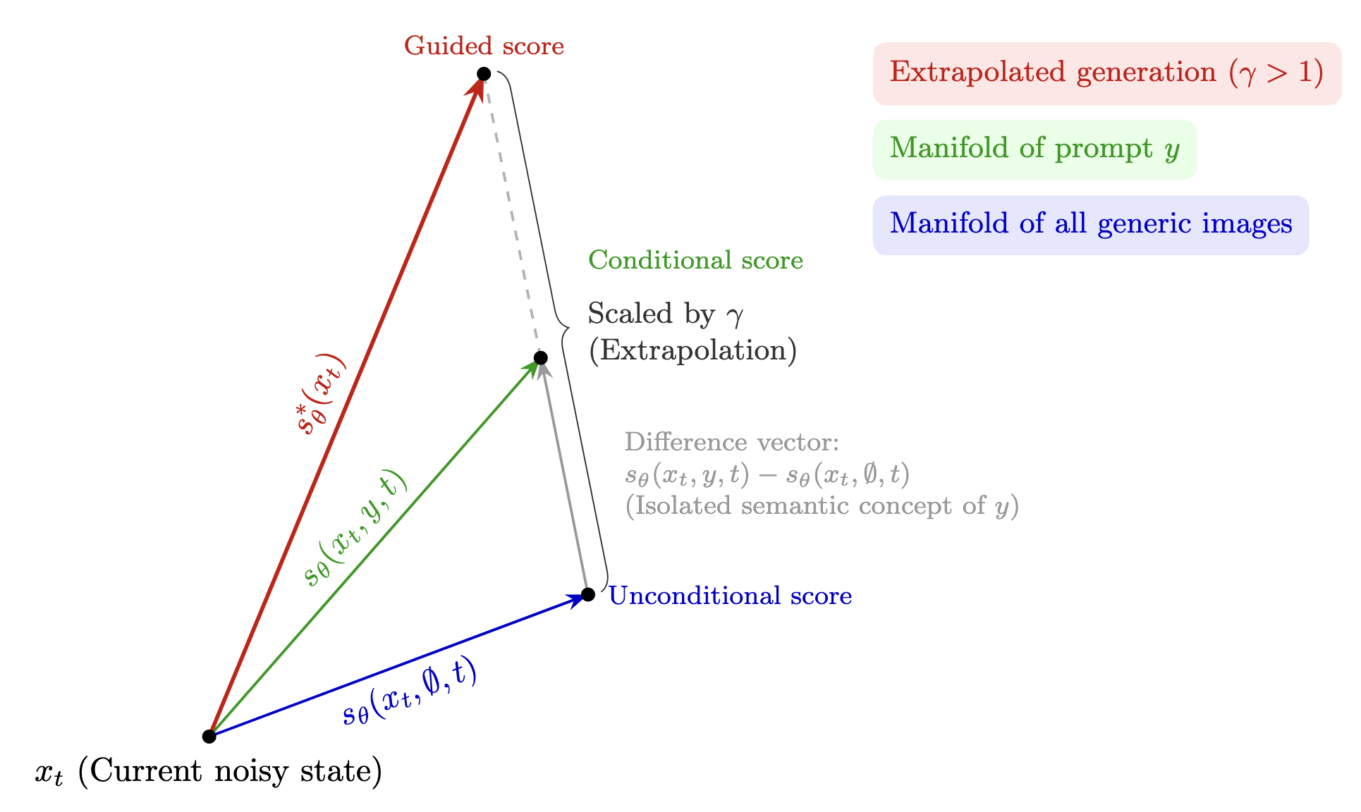
• Note that one of our intermediaries in the Section II (Assembling the CFG score) was: $$\gamma\nabla_{x_t} \log p(x_t \mid y) -(\gamma-1) \nabla_{x_t} \log p(x_t) \approx \boxed{\gamma \cdot s_\theta(x_t , y, t) - (\gamma - 1) s_\theta(x_t, \emptyset, t)}$$This format shows that CFG is simply an affine combination of the unconditional prediction and the conditional prediction (draws a straight line through two high-dimensional points).
  • If $\gamma = 0$, we are at the unconditional point.
  • If $\gamma =1$, we are at the conditional point.
  • If $\gamma > 1$, we are traveling further down that exact same straight line, past the conditional point, into extrapolated territory.

IV. Pseudocode for CFG

Because we established via Tweedie's Formula that the score is directly proportional to the negative noise: $$\nabla_{x_t} \log p(x_t) \propto -\epsilon,$$the same algebraic formula applies to noise predictions:$$s^*_\theta(x_t) = s_\theta(x_t, \emptyset, t) + \gamma (s_\theta(x_t, y, t) - s_\theta(x_t, \emptyset, t)) \implies \epsilon_\theta^* = \epsilon_\theta(x_t, \emptyset, t) + \gamma (\epsilon_\theta(x_t, y, t) - \epsilon_\theta(x_t, \emptyset, t))$$

# 1. setup & embedding
text_embeddings = clip_model.text_encode("a dog")                 # encode the conditional text → shape: [1, seq_len, dim]
empty_embeddings = clip_model.text_encode("")                     # encode empty text → shape: [1, seq_len, dim]
text_embeddings = torch.cat([empty_embeddings, text_embeddings])  # concat ^ together as the condition 
																  #     → shape: [2, seq_len, dim]

# 2. init noise to denoise w/ diffusion model
x_t = get_noise(...)                           # shape: [1, channels, height, width]

# denoising loop (sampling)
for t in tqdm(scheduler.timesteps):
	# duplicate the noisy image to match the batch size of the text embeddings
	latent_model_input = torch.cat([x_t, x_t])     # shape: [2, channels, height, width]
	
	# 3. sample from diffusion model to get noise_pred
	with torch.no_grad():
		noise_pred = model(latent_model_input, t, encoder_hidden_states=text_embeddings).sample
		# ^ because neural nets process batches in parallel on the GPU, 
		#   the diffusion model performs two entirely separate forward passes simultaneously here :0!
	noise_pred_uncond, noise_pred_text = noise_pred.chunk(2)
	
	# 4. CFG equation
	noise_pred = noise_pred_uncond + guidance_scale * (noise_pred_text - noise_pred_uncond)
	
	# 5. take one denoising step
	x_t = scheduler.step(noise_pred, t, x_t).prev_sample

1. Embeddings: text_embeddings = ...: to do CFG, we need two outputs from our model at every timestep - the conditional and unconditional output.
   • 🔑 During training, unconditional generation is learned by randomly dropping the text prompt (passing the embedding of an empty string). Conditional generation is learned by conditioning on the embedding of actual, meaningful text prompts ("a dog").
2. Initial noisy $x_T$ for the diffusion model to start from: x_t = get_noise(...); latent_model_input = torch.cat([x_t, x_t])
3. Sampling from the diffusion model: noise_pred = model(...).sample
   • Batch index 0: Model processes x_t conditioned on empty_embeddings
   • Batch index 1: Model processes x_t conditioned on text_embeddings
   • noise_pred is a tensor with a batch size of 2 containing both ^ predictions
   • .chunk(2) splits noise_pred into 2 equal parts along the batch dimension:
     • noise_pred_uncond = $\epsilon_\theta(x_t, \emptyset, t)$
     • noise_pred_text = $\epsilon_\theta(x_t, y, t)$
4. CFG math: noise_pred = noise_pred_uncond + guidance_scale * (noise_pred_text - noise_pred_uncond): $$\epsilon_\theta^* = \epsilon_\theta(x_t, \emptyset, t) + \gamma (\epsilon_\theta(x_t, y, t) - \epsilon_\theta(x_t, \emptyset, t))$$Note that here, $\epsilon_\theta^*$ is back to shape [1, channels, height, width]
5. Scheduler denoising step: x_t = scheduler.step(noise_pred, t, x_t).prev_sample: recall this step evaluates the reverse diffusion equation we derived earlier. For DDPM, that equation is: $$\begin{align*}x_{t-1} &= \mu_t + \sigma_tz, \quad z \sim \mathcal{N}(0, I) \\ &= \frac{1}{\sqrt{\alpha_t}} \left(x_t - \frac{1 - \alpha_t}{\sqrt{1 - \bar{\alpha}_t}} \epsilon_\theta^*(x_t, t)\right) + \sigma_t z\end{align*}$$

---

(Notes above this line were guided by the following blog post: https://medium.com/@baicenxiao/understand-classifier-guidance-and-classifier-free-guidance-in-diffusion-model-via-python-e92c0c46ec18)

Fancier versions of CFG

Below are my notes from a CSAIL thesis defense in February 2026. General outline: Covers the mathematical flaws of standard CFG and proposes measure-theoretic fixes (classifier-thresholded guidance, piecewise-linear diffusion, dual-reward finetuning) to allow for logical composition (AND, NOT, XOR) without destroying the data manifold.

I. Flaws of CFG

Core intuition before we dive into the math: The central goal of a generative model is to learn some function that, given a bag of inputs (e.g., images) that has some prior distribution $P_0$, learns to output $x \sim P_0(x)$, i.e. samples within this data distribution. Diffusion models approach this task by learning some function $x_{t-1} \sim f_t(x_t, t) \approx P_t(x_t)$, that aims to model the distribution $P_t = P_0 + t \text{ steps of Gaussian noising}$. If we can learn a model $f_\theta(x_t, t)$ that perfectly models $P_t(x_t)$ across all timesteps $t = T \ldots 0$, then we can create new samples $x \sim P_0(x)$ via iterative denoising: $$x_T \sim P_T = \mathcal{N}(0, I) \rightarrow x_{T-1} \rightarrow \cdots \rightarrow x_1 \rightarrow x_0 \sim P_0$$But how do we train a model to approximate $P_t$? The immediate answer might be - integrate the difference between the true $P_t(x_t)$ and our model's predicted $f_\theta(x_t, t)$ over all $x_t$'s (noisy images at this timestep). This is intractable, as there are infinite $x_t$'s in the universe. Instead, we can train a model $v_\theta(x_t, t)$ to approximate the velocity field $v_t(x) = \nabla_x P_t$.

• Q: Why are "velocities" (scores) tractable when $P_t$ is not?
  • A: This is the foundational "magic trick" of score-based generative modeling (JMLR 2005)!
    • Complex probability distributions are often members of the exponential family, i.e. can be written as $$P(x) = \frac{e^{-\text{Energy}(x)}}{Z}$$where $Z$ is the partition function, representing the total volume of all possible states in the universe to ensure all probabilities sum up to 1. Calculating $Z$ requires integrating over every possible image that could ever exist - $Z$ is mathematically intractable to compute!
    • But now let's examine the gradient of the log probability (the score function): $$\nabla_{x} \log P(x) = \nabla_x \log \left(\frac{e^{- \text{Energy}(x)}}{Z}\right) = \nabla_x (- \text{Energy}(x)) - \nabla_x \log (Z)$$Because $Z$ is a constant w.r.t. $x$, its gradient is 0. So we end up with: $\nabla_x \log P(x) = - \nabla_x \text{Energy}(x)$. The intractable $Z$ vanishes!
• Q: How can we recover new samples $x \sim P_0$ from a model $v_\theta (x_t, t)$ that has learned $\nabla_x \log P_t(x)$ across all timesteps $t$?
  • A: We do numerical integration, a fancy way of saying we take tiny steps - during inference, we
    1. Start at timestep $T$: generate a completely random matrix of pure Gaussian noise.
    2. Feed the noisy image $x_t$ and current time $t$ into the trained neural network: $v' = v_\theta(x_t, t)$. Essentially, the model looks at the noise and outputs the score, which says - "to get a slightly more realistic image, move in this exact direction $v'$."
    3. Instead of solving an integral, we use numerical integration: taking the current position, add the velocity vector multiplied by a tiny slice of time $\Delta t$. $$x_{t - \Delta t} = x_t + (\text{step\_size} \times \text{slope})$$We now have an image that is slightly less noisy: $x_{t - \Delta t}$. Rinse and repeat Steps (2) & (3) until we get a clear image!
• 💡 Essentially, diffusion models work by saying - we never need to know the shape of the entire mountain $P_t$. We don't need to build the full map; we just need a reliable compass to navigate to hills within the mountain $P_t$. The trained neural network is that compass!

So we've established that, while it is intractable to train a model $f_t \approx P_t$, we can train a model $v_t \approx \nabla_x \log P_t$. CFG essentially works by overlaying vector fields: in CFG, we take the unconditional slope $\nabla_x \log P_t (x_t)$ and the conditional slope $\nabla_x \log P_t (x_t \mid y)$. We push the generation away from the generic path and further down the specific path by doing vector math: $$v^* = s_\gamma \approx \text{new vector} = \text{unconditional vector} + \gamma \times (\text{conditional vector} - \text{unconditional vector})$$($s_\gamma$ is notation for the CFG-guided score², which is conceptually identical to $v^*$). During generation, the SDE/ODE solver (DDIM, Euler, etc.) acts like a blindfolded hiker. It asks the neural network $v^*$, "which way is uphill?" The network gives it the CFG-modified vector, and the hiker takes a tiny step. It repeats this num_inference_timesteps number of times until it reaches the top (ideally, a hill where $P_0$ is high, i.e. a clear image).

• ⚠️ Crucially: The solver never asks if a coherent mountain actually exists; it just blindly follow the local arrows.
  • Therefore, when we artificially manipulate the arrows using $\gamma$ in CFG, we risk creating a vector field that will lead us to run off the $P_t$ landscape. We need to prove that our new vector field $s_\gamma (x_t)$ actually corresponds to a valid, implied probability density $\tilde{P}_t(x_t)$. Let's investigate this next!

1. In CFG, the modified score function at a time $t$ is a weighted mean in score space: $$s_\gamma(x_t) = (1 - \gamma) \nabla_{x_t} \log P_t(x_t) + \gamma \nabla_{x_t} \log P_t (x_t \mid y)$$(To unify with the notation we were using earlier: the above equation is identical to $\gamma\nabla_{x_t} \log p(x_t \mid y) -(\gamma-1) \nabla_{x_t} \log p(x_t)$.)
2. If we integrate this score function to find the probability density $\tilde{P}_t$ it corresponds to in data space, we get: $$\tilde{P}_t(x_t) \propto P_t(x_t)^{1 - \gamma} P_t(x_t \mid y)^\gamma = P_t(x_t) \left(\frac{P_t(x_t \mid y)}{P_t(x_t)}\right)^\gamma$$By Bayes theorem, $\frac{P_t(x_t \mid y)}{P_t(x_t)} \propto P_t(y \mid x_t)$ (by a factor of $P_t(y)$), so CFG mathematically induces a probability distribution of the below form: $$\boxed{\tilde{P}_t (x_t) \propto P_t(x_t) P_t(y \mid x_t)^\gamma}$$This $\tilde{P}_t$ is the distribution our neural network is actually targeting (i.e., trying to learn) when we run the CFG code noise_pred_uncond + guidance_scale * (noise_pred_text - noise_pred_uncond)

---

[RETURN TO THESE NOTES LATER - I'm getting stuck on the math from hereon]

1. Q: Is
   • Valid process: If you take a dataset, add noise to it according to the laws of physics (the heat equation) until it is pure static, and then reverse that exact physical process, you are mathematically guaranteed to reconstruct the true dataset.
   • Invalid process: "Invalid" means that there is no forward physical process that starts at your clean images and

In the realm of

Standard CFG uses a guidance scale $\gamma$.

• $\gamma$ too low: under-steering (ignores prompt)
• $\gamma$ too high: over-saturation, diversity loss, generates "off the manifold"

What does off the manifold mean?

• In CFG, the modified score function at a time $t$ is a weighted mean in score space: $$s_\gamma(x_t) = (1 - \gamma) \nabla_{x_t} \log P_t(x_t) + \gamma \nabla_{x_t} \log P_t (x_t \mid y)$$(To unify with the notation we were using earlier: the above equation is identical to $\gamma\nabla_{x_t} \log p(x_t \mid y) -(\gamma-1) \nabla_{x_t} \log p(x_t)$.)
  • 📍 What is $P_t$?³ Imagine the universe of all possible images.
    • At $t = 0$: $P_0(x_0)$ is the distribution of perfectly clean, real images (e.g., the actual dataset). If we pick a random point in this high-dimensional point, $P_0$ is very high if the point looks like a real image (e.g., a dog!), and zero if the point looks like static noise.
    • At $t = T$: $P_T(x_T)$ is the distribution of pure, unstructured Gaussian noise: $\mathcal{N}(0, I)$.
    • At intermediate $t$: $P_t(x_t)$ is the distribution of the dataset after it has been corrupted by exactly $t$ steps of noise.
    • 🔑 Summary: given some image $x_t$, the mathematical function $P_t$ outputs a single number answering the question: "Given the exact noise level at time $t$, how likely is it that this ($x_t$) specific arrangement of pixels and static exists in our corrupted dataset?"
    • Mathematically: In diffusion, $P_t(x_t)$ is defined as the integral of the forward diffusion process applied to the true data distribution: $$P_t(x_t) = \int q(x_t \mid x_0) P_0(x_0) \, dx_0$$where $P_0(x_0)$ is the clean data, and $q(x_t \mid x_0)$ is the Gaussian transition kernel (the formula that adds $t$ steps of noise to a clean image).
      • ^ this integral says, "to find the probability of seeing this noisy image $x_t$, we must check every single clean image in the universe ($x_0$), multiply by the probability that the clean image $x_0$ could have degraded into our specific noisy image $x_t$, and sum it all up." This should sound really intractable !
    • 💡 In diffusion models, we never actually calculate $P_t(x_t)$ because summing over the entire universe of images is computationally impossible. Instead, we care about its score: $\nabla_{x_t} \log P_t (x_t)$.
      • Even though $P_t(x_t)$ is intractable, its gradient (the score) can be learned by a neural network. When the diffusion model architecture (e.g., U-Net) predicts the noise $\epsilon_\theta (x_t, t)$, it is mathematically predicting this exact gradient $\nabla_{x_t} \log P_t(x_t)$ (recall Tweedie's Formula!).
      • Conceptually: the vector $\nabla_{x_t} \log P_t(x_t)$ points toward the regions of high-dimensional space where $P_t$ is denser (where the real, corrupted images are).
• \
• If we integrate this score function to find the probability density it corresponds to in data space, we get: $$\tilde{P}_t(x_t) \propto P_t(x_t)^{1 - \gamma} P_t(x_t \mid y)^\gamma = P_t(x_t) \left(\frac{P_t(x_t \mid y)}{P_t(x_t)}\right)^\gamma$$By
  • "Data space": this is the probability density landscape $P_t$ → every possible arrangement of pixels is a coordinate $x_t$, and the altitude at any given coordinate is the probability density $P_t(x_t)$
  • "Score space": imagine you are dropped onto the landscape ^ $P_t$, but you are blindfolded - you cannot see the altitude $P_t(x_t)$, but you can feel the slope of the ground beneath your feet.
    • Score function $\nabla_{x_t} \log P_t(x_t)$ is a mathematical vector that points directly uphill toward the steepest ascent. The collection of all these vectors across the entire map is the score space!

Footnotes

1. Assuming we're working with images ↩

2. Introducing this notation now to prepare for the next section! ↩

3. Covered earlier in these notes, but we'll review here real quick. ↩