IKDiffuser is a diffusion-based generative IK solver for kinematic trees.

• $N$ = total number of end-effectors
• $e_i$ = target pose for the $i$-th end-effector
• $z$ = noisy latent variable (since this is a diffusion model)
• $\hat{q}$ = predicted joint configuration

Intuition behind their use of the transformer architecture

• "Rather than concatenating all target end-effector poses into a fixed-length vector, we represent them as a sequence of conditioning tokens."
  • Vanilla concatenation: $C_\text{fixed} = \begin{bmatrix} e_1 & e_2 & \cdots & e_N \end{bmatrix} \in \mathbb{R}^{N \times d}$
    • The neural network requires this exact input size: $q = \text{MLP}(z, C_\text{fixed})$
    • ⚠️ If $e_2$ (e.g., the right hand target) is missing or undefined, the dimension of $C_\text{fixed}$ breaks :"(. The network expects $N \times d$ values, and if we input "dummy" zeros, performance degrades / OOD for model.
• 💡 "Attention mechanism implicitly infers inter-branch dependencies and constraints entirely from the data, regardless of the number of end-effectors."
  • 🔑 Instead of a fixed vector, the target poses are treated like a sequence of words (tokens), where the length of the sentence can vary.
  • Concretely:
    • Each provided pose $e_i$ is mapped to a high-dimensional token $t_i$
    • Because sequence order doesn't tell the network which end-effector is which (need to embed $i$), an identity/structural encoding $p_i$ is added: $t_i = \text{Linear}(e_i) + p_i$
    • The condition is now a sequence of $k$ available tokens, where $k \leq N$: $C_\text{seq} = \{t_1, t_2, \ldots, t_k\}$
    • The network uses cross-attention to process this sequence: $\hat{q} = \text{Transformer}(z, C_\text{seq})$

N_EFFECTORS = 4
POSE_DIM = 6 # x, y, z, roll, pitch, yaw
EMBED_DIM = 128

class FixedVectorIKConditioner(nn.Module):
	def __init__(self):
		super().__init__()
		self.mlp = nn.Linear(N_EFFECTORS * POSE_DIM, EMBED_DIM)
	def forward(self, targets_dict):
		# targets_dict: {0: pose0, 1: pose1, 2: pose2, 3: pose3}
		pose_list = []
		for i in range(N_EFFECTORS):
			if i in targets_dict: pose_list.append(targets_dict[i])
			else: pose_list.append(torch.zeros(POSE_DIM)) # yikes...
		c_fixed = torch.cat(pose_list, dim=-1) # shape: [batch, 4 * 6]
		return self.mlp(c_fixed)

class TokenSeqIKConditioner(nn.Module):
	def __init__(self):
		super().__init__()
		self.pose_embedder = nn.Linear(POSE_DIM, EMBED_DIM) # 6D pose → 128D token
		# positional encoding
		self.effector_id_embeddings = nn.Embedding(N_EFFECTORS, EMBED_DIM)
	def forward(self, targets_dict):
		tokens = []
		for effector_id, pose in targets_dict.items():
			pose_feat = self.pose_embedder(pose) # shape: (128)
			id_feat = self.effector_id_embddings(torch.tensor(effector_id)) # shape: (128)
			token = pose_feat + id_feat
			tokens.append(token)
		c_seq = torch.stack(tokens, dim=1) # (batch, num_available_tokens, 128)
		# TODO: pass to cross-attention layer in the diffusion model
		# attention mechanism natively accepts variable-length sequences
		return c_seq

Masked marginalization training strategy TLDR

• Masked marginalization strategy during training that enforces constraints on specified end-effectors while treating the remaining ones as latent.
• 💡 Core idea: During inference, we want to be able to only specify target end-effector poses for a subset of the full number of end-effectors the model was trained on (& do so for dynamic subsets)
  • ❓ Does transformer architecture not inherently do this? No, we need to separate "plumbing" from "intelligence."
    • Cross-attention mechanism purely solves a computational constraint: it allows the math to compute without throwing a RuntimeError: tensor size mismatch regardless of how many end-effector target poses we feed in. But attention does not encode kinematics!
    • Masked marginalization during training solves a statistical/knowledge constraint.
      • If we used a transformer but did not use masked marginalization during training (i.e. always fed the network all $N$ end-effectors during every training step), here is what would happen during inference: 1. You provide only 1 target (e.g. left hand) 2. The plumbing works: the cross-attention layer happily accepts the single token, matrices all multiply, code runs wo crashing... 3. The network outputs absolute garbage for all the non-specified targets. Because the network suffers from a massive OOD shock! - During its entire training life, it learned that finding a valid joint configuration q required balancing the constraints of four targets. It never learned the kinematic priors of how a human/robot arm hangs naturally when unconstrained. It never learned how to guess or "hallucinate" valid joint angles for missing limbs because it never had to.
      • ^ to fix this: masked marginalization during training!

Guidance TLDR (classifier guidance, not CFG)

• Supports integration of task-specific objectives through guidance at inference time (without retraining)
  • Manipulability maximization (Jacobian objective)
  • Warm-start initialization

Paper summary

• 📍 Results: When used to seed an optimization-based IK solver, IKDiffuser can boost the success rate of finding feasible solutions (within $10^{-3}$ mm and $10^{-3}$ deg precision) on the 29-DoF Unitree G1 humanoid:
  • Success rate: 21.01% → 96.96%
  • Time: 1830 ms to 280 ms for 128 feasible solutions
    • (might have some amortization going on? or subtracting time it takes to spin up program / my machine might have more overhead time spinning up programs)
• 🔑 Contributions of paper:
  1. Diffusion-based generative IK solver
  2. Structure-agnostic conditioning to allow variable num of end-effector goals
  3. Guided sampling strategy w task-specific objectives
  4. Masked marginalization strategy during training - enables enforcing only a specified number of end-effector poses
  5. Extensive benchmarking against optimization + learning based baselines
  6. Open-sourcing code at some point

Transformer architecture specifics

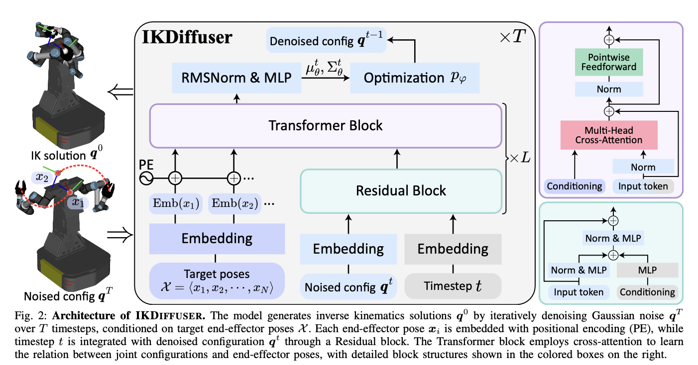
Model predicts $\epsilon_\theta(\cdot)$

• Key architecture components:
  • Multi-headed cross-attention transformer block
    • Cross-attention mechanism captures the correlation between joint configs and end-effector poses
  • Each end-effector pose $x_i$ is encoded with a positional encoding to form the keys + values in transformer
  • Query is obtained from time-conditional noised configuration produced by a residual block that jointly embeds the noised joint configuration $q^t$ and timestep $t$
  • Since the joint configuration is a single "token" sequence, self-attention is unnecessary in the transformer block
• At each inference step:
  1. The model estimates the diffusion noise $\epsilon_\theta^t$ by applying cross-attention between the target end-effector poses and the time-conditional noised configuration.
  2. $\mu_\theta^t$ and $\Sigma_\theta^t$ of the reverse diffusion prior are computed from $\epsilon_\theta^t$: $$\begin{align*}\mu_\theta(q^t, X, t) &= \frac{1}{\sqrt{\alpha^t}} \left(q^t - \frac{1 - \alpha^t}{\sqrt{1 - \bar{\alpha}^t}}\epsilon_\theta(q^t, X, t)\right) \\ \Sigma_\theta (q^t , X, t) &= \frac{1 - \bar{\alpha}_{t-1}}{1 - \bar{\alpha}_t} \beta_t I\end{align*}$$
  3. Denoised joint configuration $q^{t-1}$ is sampled following Equation 16:
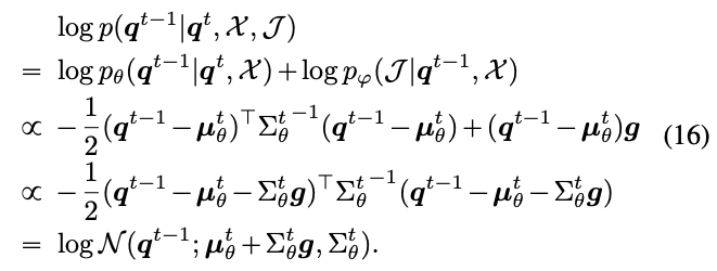
     • where gradient $g$ steers the process toward satisfying optimization objectives

Implementation details

[From chatting with Gemini]

• 💡 The core engine of any transformer is scaled dot-product attention: queries $Q$, keys $K$, values $V$ $$\text{Attention} (Q, K, V) = \text{softmax} \left(\frac{QK^\top}{\sqrt{d_k}}\right)V$$In multi-head attention, we project $Q, K, V$ into $h$ smaller subspaces (heads), perform attention in parallel, concatenate the results, and project back: $$\text{head}_i = \text{Attention} (QW_i^Q, KW_i^K, VW_i^V) \rightarrow \text{MHA}(Q, K, V) = \text{Concat}(\text{head}_1, \ldots, \text{head}_h) W^O$$ where $W_i^Q \in \mathbb{R}^{d \times d_k}, W_i^K \in \mathbb{R}^{d \times d_k}, W_i^V\in \mathbb{R}^{d \times d_v}$ and $W^O\in \mathbb{R}^{d_v \times d}$
  • Typically $d_k = d_v = d/h$
• Cross-attention in IKDiffuser:
  • In standard NLP setups, $Q,K,V$ are all sequences of many tokens (sentences!)
  • In IKDiffuser, the setup is asymmetric: Let $N$ be the number of provided end-effector targets, and $d$ be the embedding dimension.
  1. The conditioning tokens: (keys & values) Each target pose $x_i$ is passed through an embedding layer and added to a positional encoding ($PE$) to identify which end-effector it is. This forms a sequence of length $N$: $$E_X = \begin{bmatrix} \text{Emb}(x_1) + PE_1 & \ldots & \text{Emb}(x_N) + PE_N\end{bmatrix} \in \mathbb{R}^{N \times d}$$ $K = E_X W^K \in \mathbb{R}^{N \times d}, V = E_X W^V \in \mathbb{R}^{N\times d}$
  2. The noised configuration: (query) The current noised joint config $q^t$ and the timestep $t$ are processed by a residual block into a single feature vector: $$q_\text{embed} = \text{ResidualBlock}(q^t, t) \in \mathbb{R}^{1 \times d}$$ $Q = q_\text{embed} W^Q \in \mathbb{R}^{1 \times d}$
  3. The cross-attention operation: $Q K^\top \implies (1 \times d) \times (d \times N ) = (1 \times N)$
     • $(1 \times N)$ represents the attention scores → "Given the current state of the whole robot ($Q$), how much should I care about the left hand vs. right foot ($K$) to figure out the next denoising step?"
     • Then multiply by $V$: $\text{softmax} (1 \times N) \times (N \times d) = (1 \times d)$

class IKDiffuserTransformerBlock(nn.Module):
	def __init__(self, embed_dim=128, num_heads=8):
		super().__init__()
		self.embed_dim = embed_dim
		# Cross attention
		self.cross_attn = nn.MultiheadAttention(embed_dim, num_heads, batch_first=True)
		self.norm1 = nn.LayerNorm(embed_dim)
		# Pointwise feedforward (standard transformer MLP)
		self.ffn = nn.Sequential(
			nn.Linear(embed_dim, embed_dim * 4),
			nn.GELU(),
			nn.Linear(embed_dim * 4, embed_dim)
		)
		self.norm2 = nn.LayerNorm(embed_dim)
	def forward(self, q_t_embed, cond_tokens):
		"""
		q_t_embed: (batch, 1, embed_dim) → query (joints + timestep)
		cond_tokens: (batch, N, embed_idm) → keys/values (target poses)
		"""
		# Cross attention
		attn_out, _ = self.cross_attn(
			query=q_t_embed,
			key=cond_tokens,
			value=cond_tokens
		)
		# Residual connection + norm
		x = self.norm1(q_t_embed + attn_out)
		# Feed forward
		ffn_out = self.ffn(x)
		# Residual connection + norm
		out = self.norm2(x + ffn_out)
		return out # shape: (batch, 1, embed_dim)

[TODO ^ READ INTO THIS MORE]

Intuition

• Query ($Q$): What you type into the search bar ("I need a book about flowers")
• Key ($K$): The title or tags on the spine of the book on the shelf ("Roses: How to Garden")
• Value ($V$): The actual pages and content inside the book (the text you read)
• 💡 You compare your query to all the keys. When you find a strong match, you retrieve the value of that specific book.

NLP intuition: self-attention

Core problem that self-attention solves: words are ambiguous! A word needs context from its neighbors to figure out what it actually means. In NLP, a sentence uses self-attention, meaning every word acts as a $Q, K, V$ simultaneously.

• Example: "The bank of the river." Imagine the network is currently trying to process the word bank. It needs to figure out if it's a financial institution or the side of a body of water.
  1. Query: The word "bank" generates a query. It essentially shouts to the rest of the sentence - "I am 'bank.' I need clues about money or water. What do you guys have?"
  2. Keys: Every other word in the sentence holds up a key (a nametag):
     • "The" holds up a key: "I am an article."
     • "river" holds up a key: "I am water, flowing, nature..."
  3. The match ($Q \times K^\top$): The network calculates the compatibility between "bank"'s query and everyone else's keys. The query for "bank" strongly aligns with the key for "river." The attention score is large!
  4. The value: Now that "bank" knows it should pay attention to "river," it absorbs the actual substance (the value) of the word "river."
  • ^ the result: the word "bank" updates its internal math to mean "riverbank" instead of "JPMorgan."

IKDiffuser intuition: cross-attention

In IKDiffuser, we are using cross-attention: the query comes from one place, but keys and and values come from somewhere else. We aren't comparing a sentence to itself - we are comparing a robot to its targets.

• Example: Assume the robot is currently in a random noisy scrambled pose, and it has two targets: a left hand target (pick up a cup) and a right foot target (step on a pedal)
  1. Query: The robot's current state → the entire current, messy state of the robot (all 20smth of its joints mashed into one embedding) generates a single query
     • The robot asks - "I am currently at timestep $t$. I need to figure out how to un-scramble myself into a valid pose. Which targets should my specific joints be listening to?"
  2. Keys: The target labels → the target end-effector poses hold up their keys (tokens combined with a positional encoding)
     • Target 1 key: "I am the left hand goal. I am located at coordinate $(x, y, z)$"
     • Target 2 key: "I am the right foot goal. I am located at coordinate $(a, b, c)$"
  3. The match ($Q \times K^\top$): The network compares the robot's query to the target keys (the network's weights have learned anatomy)
     • The "left shoulder" part of the robot's query should strongly match with the "left hand" key
     • The "left shoulder" part of the robot's query should largely ignore the "right foot" key
  4. The value: Once the left shoulder realizes it needs to pay attention to the left hand target, it pulls in the value of that target.
     • The value contains the spatial features required to actually pull the arm in that direction.

Objective-guided sampling (how to guide sampling at inference time - Section D)

• 💡 This section establishes the mathematical mechanisms behind objective-guided sampling: it proves that if you have any arbitrary objective function, you can steer the diffusion process by taking the derivative of that function and shifting the Gaussian mean (aka., how to steer IKDiffuser)
  • Section E (next section - Task-specific objectives) defines the actual rules IKDiffusion enforces out-of-the-box (aka., directions IKDiffuser can steer toward)

IKDiffuser uses classifier guidance! The standard classifier guidance shifts the predicted score (or mean) using the gradient of the classifier: $$\hat{\mu} = \mu + \Sigma \nabla_x \log p(y \mid x)$$We'll see some formulation of the above formula pop up multiple times throughout these notes! e.g., $\mu_\theta^t + \Sigma_\theta^t g$.

Math

Use Bayes' rule to combine the learned diffusion model with custom rules. "To solve the IK problem, IKDiffuser samples from the posterior distribution $p(q^0 \mid X, J)$, which is decomposed into the diffusion prior $p_\theta(q^0 \mid X)$ and the task-specific constraint likelihood $p_\varphi (J \mid q^0, X)$."

• 💡 Goal: We want to sample from the guided distribution $p(q^{t-1} \mid q^t, X, J)$, which is proportional to the prior multiplied by the objective likelihood.
  • "We incorporate the differentiable objectives $J$ into the reverse diffusion process by combining the learned denoising step $p_\theta(q^{t-1} \mid q^t, X)$ with the constraint likelihood at each timestep $t$:" $$p(q^{t-1} \mid q^t , X, J) \propto p_\theta(q^{t-1} \mid q^t , X) \cdot p_\varphi(J \mid q^{t-1}, X)\qquad \qquad (14)$$Full Bayes: $$p(q^{t-1} \mid q^t, X, J) =

\frac{
p_\theta(q^{t-1} \mid q^t, X), p_\varphi(J \mid q^{t-1}, X)
}{
\textcolor{blue}{
\displaystyle \int p_\theta(\tilde q^{,t-1} \mid q^t, X), p_\varphi(J \mid \tilde q^{,t-1}, X), d\tilde q^{,t-1}
}
}$$Blue part is dropped in $(14)$. This is valid in this use case because we write $p(q^{t-1} \mid \ldots) \propto \ldots$, and the denominator is independent of $q^{t-1}$ (so is just some scalar constant relative to the distribution $p(q^{t-1})$). Also, later when we do $\nabla \log p$, constants will disappear anyways (gradient is 0).

• ^ Note that this decomposition is entirely just Bayes rule: $$p(q^0 \mid X, J) = \frac{p(J \mid q^0, X)p(q^0 \mid X)}{p(J \mid X)}$$and then we defined $p_\theta(q^0 \mid X)$ = learned prior (diffusion model), $p_\varphi(J \mid q^0, X)$ = likelihood encoding task constraints
• To make the math easier, we work in the log space: $$\log p(q^{t-1} \mid \ldots) = \log p_\theta(q^{t-1} \mid \ldots) + \log p_\varphi(J \mid q^{t-1}, \ldots)$$Notice that because multiplying probabilities becomes adding their logs, combining multiple custom objectives is very easy in the IKDiffuser setup!
• 🔑 Math steps for incorporating the custom objective probability distribution into the diffusion denoising prior: TL;DR, use Taylor expansion to approximate the objective, then merge with learned $p_\theta$!

1. The Taylor expansion (approximating the objective):
   • ⚠️ The objective likelihood $p_\varphi$ could be highly non-linear and complex (e.g., a collision-checking function). To make it mathematically compatible with the Gaussian diffusion model, we approximate it locally using Taylor expansion.
     • Because the diffusion step is tiny, $q^{t-1}$ will be very close to the model's predicted mean $\mu_\theta^t$. \
       • Given that $p_\theta(q^{t-1} \mid q_t, X)$ is Gaussian (by typical diffusion setup), its mass is concentrated near the mean: $\mu_\theta^t = \mu_\theta(q^t, X, t)$.
     • So we perform a first-order Taylor expansion of the log-likelihood around $\mu_\theta^t$: $$\log p_\varphi(J \mid q^{t-1}) \approx \text{constant} + (q^{t-1} -\mu_\theta^t)^\top g$$where $g$ is the gradient of the objective evaluated at the mean: $g = \nabla_q \log p_\varphi(J \mid q)\big|_{q = \mu_\theta^t}$
       • We can drop constants because in the world of PDFs, a static number added in the log-space is just a normalization constant. Because a probability distribution must always sum/integrate to $1.0$, $Z$ is always whatever scaling number required to make the area under the curve equal to 1. It doesn't change where the peak of the bell curve is (the mean) or how wide it is (the variance). So when we get these constants, we just drop them (as in ignore keeping track of them).
   • 🔑 Written out in full: $$\log p_\varphi(J \mid q^{t-1} , X) \approx \log p_\varphi (J \mid \mu_\theta^t , X) + (q^{t-1} - \mu_\theta^t) g,\quad \text{where } g = \nabla_{q^{t-1}} \log p_\varphi (J \mid q^{t-1} , X) \big|_{q^{t-1} = \mu_\theta^t} \qquad (15)$$where $\log p_\varphi ( J \mid \mu_\theta^t, X)$ is a constant, $\mu_\theta^t = \mu_\theta(q^t, X, t)$ is the inferred params of original diffusion process.
   • 💡 (Note to self:) This could be a cool place to explore using a function that uses Gemini / VLM to make a collision-avoidance objective to bias the IK! [Look into making differentiable functions that involve LLM outputs]
2. Expanding the Gaussian prior: We know the diffusion prior $p_\theta$ is a Gaussian $\mathcal{N}(\mu_\theta^t, \Sigma_\theta^t)$. The log of a Gaussian (ignoring normalizing constants) is: $$\log p_\theta \propto -\frac{1}{2} (q^{t-1} - \mu_\theta^t)^\top \Sigma_\theta^{t-1} (q^{t-1} - \mu_\theta^t)$$(^ this is the Mahalanobis distance, a measure of the distance between a point $P$ and a probability distribution $Q$. Here, we have the negative of the distance between $q^{t-1}$ and the diffusion prior)
3. Merging: Now we add Step 1 and Step 2 together: $$\log p(q^{t-1} \mid \ldots) \propto \underbrace{- \frac{1}{2} (q^{t-1} - \mu_\theta^t)^\top \Sigma_\theta^{t-1} (q^{t-1} - \mu_\theta^t)}_{\text{Step 2}} + \underbrace{(q^{t-1} -\mu_\theta^t)^\top g}_\text{Step 1, constant dropped}$$This looks messy, but we can complete the square to obtain the guided transition kernel: $$\begin{align*}

\log p(q^{t-1}\mid \cdots) &\propto -\tfrac{1}{2}(q^{t-1}-\mu_\theta^t)^\top \Sigma_\theta^{t^{-1}} (q^{t-1}-\mu_\theta^t) + (q^{t-1}-\mu_\theta^t)^\top g \ &= -\tfrac{1}{2}\Big[(q^{t-1})^\top \Sigma_\theta^{t^{-1}} q^{t-1} - 2 (q^{t-1})^\top \Sigma_\theta^{t^{-1}} \mu_\theta^t + (\mu_\theta^t)^\top \Sigma_\theta^{t^{-1}} \mu_\theta^t\Big] + (q^{t-1})^\top g - (\mu_\theta^t)^\top g \ &= -\tfrac{1}{2}(q^{t-1})^\top \Sigma_\theta^{t^{-1}} q^{t-1} + (q^{t-1})^\top \Sigma_\theta^{t^{-1}} \mu_\theta^t + (q^{t-1})^\top g + \text{const} \ &= -\tfrac{1}{2}(q^{t-1})^\top \Sigma_\theta^{t^{-1}} q^{t-1} + (q^{t-1})^\top\big(\Sigma_\theta^{t^{-1}} \mu_\theta^t + g\big) + \text{const} \ &= -\tfrac{1}{2}\Big[(q^{t-1})^\top \Sigma_\theta^{t^{-1}} q^{t-1} - 2 (q^{t-1})^\top\big(\mu_\theta^t + \Sigma_\theta^t g\big) + (\mu_\theta^t + \Sigma_\theta^t g)^\top \Sigma_\theta^{t^{-1}} (\mu_\theta^t + \Sigma_\theta^t g)\Big] + \text{const} \ &= -\tfrac{1}{2}\big(q^{t-1} - (\mu_\theta^t + \Sigma_\theta^t g)\big)^\top \Sigma_\theta^{t^{-1}} \big(q^{t-1} - (\mu_\theta^t + \Sigma_\theta^t g)\big) + \text{const} \ &= \log \mathcal{N}!\left(q^{t-1};\ \mu_\theta^t + \Sigma_\theta^t g,\ \Sigma_\theta^t\right). \end{align*}$$This is the exact formula for the log a new Gaussian distribution!$$\boxed{\log \mathcal{N}(q^{t-1}; \mu_\theta^t + \Sigma_\theta^t g, \Sigma_\theta^t)}$$

• 📍 Conclusion: To apply complex, custom constraints during inference, we take the mean predicted by our neural network ($\mu_\theta^t$), calculate the gradient of the objective ($g$), then scale it by the variance $(\Sigma_\theta^t)$ and shift the mean to perform guided sampling.

Pseudocode

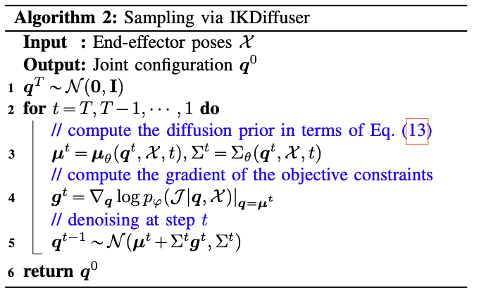
def sample_with_guidance(model, targets_dict, custom_objective_fn, num_steps=1000):
	"""
	targets_dict: The end-effector goals (X)
	custom_objective_fn: A function that takes joint angles and returns a scalar (J)
						→ e.g. higher score = further away from obstacles
	"""
	batch_size = 1
	q_t = torch.randn(batch_size, model.num_joints) # q_T
	# Iterative denoising
	for t in reversed(range(num_steps)): # line 2 of alg.
		t_tensor = torch.tensor([t]) # timestep tensor
		# Compute diffusion prior
		with torch.no_grad():
			# line 3 of alg.
			mu_theta, sigma_theta = model.predict_params(q_t, targets_dict, t_tensor)
			
		mu_theta_opt = mu_theta.detach().requires_grad_(True)
		# Evaluate how well the current predicted mean satisfies our custom rule
		objective_score = custom_objective_fn(mu_theta_opt) # log p_phi(J | mu_theta, X)
		# Calculate the gradient g w.r.t. the mean (line 4 of alg.)
		# This answers: "How should I change these joint angles to increase the score?"
		g = torch.autograd.grad(outputs=objective_score, inputs=mu_theta_opt)[0]
		
		# Sample the next denoise step from the new guided Gaussian (line 5)
		# Denoising with guidance
		guided_mu = mu_theta + (sigma_theta * g)
		# q_{t-1} ~ N(guided_mu, sigma_theta)
		noise = torch.randn_like(q_t) if t > 0 else 0.0 # no noise on the last step
		std_dev = torch.sqrt(sigma_theta)
		q_t = guided_mu + (std_dev * noise) # line 5
	
	return q_t # line 6

Task-specific objectives (how IKDiffuser uses the "engine" built in Section D)

"In many practical settings, IK solutions are not uniquely characterized by end-effector pose constraints alone: different tasks may favor different regions of the configuration space, for example, prioritizing continuity with previous solutions (warm-start IK generation), maximizing manipulability (manipulability-aware IK generation), or satisfying additional safety or comfort constraints."

• 💡 Instead of retraining a separate model for every preference, IKDiffuser has a set of task-specific objectives that can be injected at sampling time as auxiliary likelihood terms whose gradients guide the diffusion process.
  • Users can also incorporate additional, customized objectives as long as they are differentiable w.r.t $q$, enabling plug-and-play control of the generated IK solutions without retraining the model.
• 📍 Using multiple objectives is easy in IKDiffuser! Because probabilities multiply, their logarithms add - so the model calculates the "pull" of objective 1, the "pull" of objective 2, etc. ... and then adds those vectors together to nudge the robot in the combined direction.

Math for combining objectives during guided sampling

If you have multiple independent objectives $J_k$, the total likelihood that a joint configuration $q$ satisfies all of them is the product of their individual likelihoods: $$p_\varphi(J \mid q^{t-1}, X) = \prod_k p_\varphi(J_k \mid q^{t-1}, X)$$When we plug this into the Taylor expansion framework ($\log p_\varphi(J \mid q^{t-1}) \approx \text{constant} + (q^{t-1} -\mu_\theta^t)^\top g$), we take the log: $$\log p_\varphi (J \mid q^{t-1}, X) = \sum_k \log p_\varphi(J_k \mid q^{t-1} , X)$$Therefore, the total guidance gradient $g$ is the sum of the individual gradients evaluated at the current mean $\mu^t$ (dropping all constants, which are locked in by the fact that $\int p = 1$ for any probability distribution $p$): $$\boxed{g = \sum_k \nabla_q \log p_\varphi(J_k \mid q) \bigg|_{q = \mu^t}}$$

TL;DR of the specific objective implementations in IKDiffuser

More detail is provided in subsequent sections.

• 📍 In the setup we have here, everything is framed as a log-likelihood ($\log p_\varphi$), so the guidance gradient $g = \nabla_q \log p_\varphi$ always points "uphill" toward higher probability. i.e., the guidance sampling we do here performs gradient ascent!
• Warm-started IK generation: It prevents the robot from flailing wildly between consecutive time frames. If the robot's arm is reaching across a table, there are infinite ways its elbow could be positioned to keep the hand in the same spot. Warm-starting forces the solver to pick the elbow position that is mathematically closest to where the elbow was one millisecond ago.
• Manipulability-aware IK generation: It prevents the robot from "locking" its knees or elbows. In robotics, a fully extended, straight arm is in a "singularity"--it loses the ability to move freely in certain directions. This objective forces the model to favor poses where the joints are bent and have maximum physical leverage to move in any 3D direction if needed.

Warm-started IK generation

• 💡 Goal: Bias the solver toward positions that are mathematically closest to the current robot joint configurations.

Define a Gaussian-like penalty based on the Euclidean distance between the current configuration $q$ and the prior frame's configuration $q_\text{prior}$: $$\log p_\varphi(J_\text{warm}\mid q, X) = -||q - q_\text{prior}||^2_2$$ To get the gradient $g_\text{warm}^t$, we take the derivative of this squared distance with respect to $q$, evaluated at the model's current predicted mean $\mu^t$: $$g_\text{warm}^t = \nabla_q \left(-||q - q_\text{prior}||^2_2\right)\bigg|_{q = \mu^t} = \boxed{-2(\mu^t - q_\text{prior})}$$(^ this is just basic calculus: the derivative of $-x^2$ is $-2x$.)

^ "Incorporating this gradient $g_\text{warm}^t$ into the sampling process yields solutions that remain close to prior configurations, enabling smooth and stable motions in practical applications without retraining the model."

Manipulability-aware IK generation

• 💡 Goal: Bias the solver to poses far away from kinematic singularities.

This uses Yoshikawa's manipulability measure.

• Let $J_i$ be the Jacobian matrix of the $i$-th arm.
• The Jacobian translates joint velocities into 3D hand velocities.
• The determinant of $J_i J_i^\top$ represents the volume of the "manipulability ellipsoid" (how freely the hand can move).
• 🔑 We want to maximize this volume ^ for all end-effectors $N_{ee}$: $$\log p_\varphi(J_\text{manip} \mid q, X)= \sum_{i=1}^{N_{ee}} \sqrt{\det(J_i J_i^\top)}$$The gradient $g_\text{manip}^t$ requires taking the derivative of this determinant w.r.t. the joint angles $q$.

Pseudocode for task specific objective-guided sampling

def calculate_warm_start_gradient(mu_theta, q_prior):
	"""
	mu_theta: Current predicted joint angles, shape: (batch, num_joints)
	q_prior: The joint angles from the previous timestep
	"""
	g_warm = -2.0 * (mu_theta - q_prior)
	return g_warm

def manipulability_objective_fn(q_tensor, robot_kinematics_model):
	"""
	Calculates Yoshikawa's measure: sum( sqrt(det(J * J^T)) )
	"""
	total_manipulability = 0.0
	# Get the Jacobian matrices for all end effectors at the current joints q
	# Shape: (num_effectors, 6, num_joints)
	jacobians = robot_kinematics_model.compute_jacobians(q_tensor)
	
	for i in range(NUM_EFFECTORS):
		J = jacobians[i]
		J_T = J.transpose(-2, -1) # transpose
		# Calculate manipulability measure
		# Add a tiny eps 1e-6 to determinant to prevent sqrt(0) → NaN gradients
		measure = torch.sqrt(torch.det(torch.matmul(J, J_T)) + 1e-6)
		total_manipulability += measure
		
	return total_manipulability
	
def compute_total_gradient(mu_theta, q_prior, robot_kinematics_model, 
							use_warm=True, use_manip=True):
	total_g = torch.zeros_like(mu_theta)
	
	# Add warm-start gradient
	if use_warm and q_prior is not None:
		g_warm = calculate_warm_start_gradient(mu_theta, q_prior)
		# Weighting factor (alpha=0.5) to control how strictly to enforce this rule
		total_g += (0.5 * g_warm)
		
	# Add manipulability gradient
	if use_manip:
		mu_opt = mu_theta.detach().requires_grad_(True)
		manip_score = manipulability_objective_fn(mu_opt, robot_kinematics_model)
		g_manip = torch.autograd.grad(outputs=manip_score, inputs=mu_opt)[0]
		# Weighting factor 0.1
		total_g += (0.1 * g_manip)
		
	return total_g
	
# Usage inside the diffusion loop from Section III(D) in IKDiffuser paper
guided_mu = mu_theta + sigma_theta * compute_total_gradient(...)

Marginal inference

• 💡 Goal: We want to train one model that is capable of performing "marginalization" on-the-fly during inference, i.e. we can feed in a variable number of target poses and the model will fill in reasonable robot configs for the under-specified joints/end-effector poses.
  • ⚠️ Would be problematic if the model outputs a completely broken left-hand target pose (i.e. penetrates robot torso oop) when only a right-hand pose is provided. We fix this by having the model learn the marginal distribution!

TL;DR: Have the model learn an empty token.

TL;DR intuition

• Instead of doing the marginalization math at inference time, we train the neural network to learn an "empty token" - invent a blank target label $x_\varnothing$
• During training: Randomly hide targets and replace them with this blank label $x_\varnothing$. The network learns that whenever it sees this label, it is free to put that limb in whatever natural, physically valid resting pose it wants.
• ❓ Why not just pass a target of all zeros?
  • If you pass $[0, 0, 0, 0, 0, 0]$ for the missing target pose, the model will interpret this as wanting the left hand at the coordinate origin - yikes!!
  • This is why the empty token must be an abstract, learnable concept $z_\varnothing$ that lives inside the neural network's latent space, not a physical coordinate.
• ⚠️ Clearing up notation: What is the difference between $x_\varnothing$ and $z_\varnothing$?
  • $x_\varnothing$ is the concept: it represents the abstract idea of "no target provided" in the physical 3D input space
  • $z_\varnothing$ is the implementation (the latent code): it is a tangible, EMBED_DIM-dim vector of floating point numbers that the neural network actually uses to represent that concept. It lives exclusively in the latent embedding space.

Math

We want the probability of a joint configuration $q^0$ given only a subset of specific targets $X_S$: $$p(q^0 \mid X_S, J) \propto \int p(q^0 \mid X, J) p(X_{\bar{S}} \mid X_S, J) \, dX_{\bar{S}} \qquad \qquad (22)$$This formula says: take the probability of the full body pose, multiply it by the probability of the missing limbs ($X_{\bar{S}}$), and integrate over every possible position $dX_{\bar{S}}$,. Because the space of possible limb positions is infinite, this integral is computationally intractable.

• 💡 Training hack: ^ Instead of integrating, we modify the training data.
  • For a full set of targets $X = \langle x_1, x_2, \ldots, x_N\rangle$, we generate a random binary mask $m$.
  • Then, construct a corrupted sequence $\tilde{X}$: $$\tilde{x}_i = \begin{cases} x_i, & m_i = 1\\ z_\varnothing, & m_i = 0\end{cases}$$
  • We train the model $p_\theta (q^0 \mid \tilde{X}, J)$ to reconstruct the full, correct body pose $q^0$ even when some $x_i$ are replaced by $z_\varnothing$.
  • 🔑 By doing this over millions of iterations, the neural network learns to perform the intractable integral from Equation $(22)$ inside its own weights.
• 📍 At inference time: When the user actually wants to use the model and only provides a target for the right hand (subset $S$), we build the sequence using the learned latent code $z_\varnothing$: $$\tilde{x}_i = \begin{cases} x_i, & i \in S\\ z_\varnothing, & i \notin S\end{cases}$$The sequence length remains exactly $N$ - the math flows into the cross-attention layers, and the model outputs a full-body pose where the unconstrained limbs look statistically natural.

Pseudocode

class IKDiffuserConditioner(nn.Module):
	def __init__(self):
		super().__init__()
		self.pose_embedder = nn.Linear(POSE_DIM, EMBED_DIM) # 6D pose → 128D token
		# Learned empty token
		self.empty_token = nn.Parameter(torch.randn(1, 1, embed_dim)) # shape: (128)
		# Positional encoding
		self.effector_id_embeddings = nn.Embedding(N_EFFECTORS, EMBED_DIM)
		
	def forward(self, target_poses, drop_mask=None):
		"""
		target_poses: Shape (batch_size, N, pose_dim)
		drop_mask: Shape (batch_size, N). True if effector should be dropped/is missing.
		"""
		batch_size = target_poses.shape[0]
		
		# Embed all continuous poses first: (batch_size, N, 128)
		pose_embeddings = self.pose_encoder(target_poses)
		
		# Apply the marginalization mask
		if drop_mask is not None:
			# Expand the empty token to match the batch size: (B, 1, 128) → (B, N, 128)
			empty_tokens_expanded = self.empty_token.expand(batch_size, N_EFFECTORS, -1)
			# Expand the drop mask so it can broadcast over embedding dimension
			drop_mask_expanded = drop_mask.unsqueeze(-1) # (batch_size, N, 1)
			# If drop mask is True, use empty_tokens_expanded. Otherwise, use pose_embeddings.
			marginalized_embeddings = torch.where(
				drop_mask_expanded,
				empty_tokens_expanded,
				pose_embeddings
			)
		else: # No dropping / not learning marginalization
			marginalized_embeddings = pose_embeddings
		
		# Add structural identity (whcih token is the left hand vs. right foot, etc.)
		final_tokens = marginalized_embeddings + self.positional_encodings
		
		# Pass to cross-attention layer
		return final_tokens

# Training example: Generate a random mask where ~20% of effectors are True (dropped)
conditioner = IKDiffuserConditioner()
drop_mask = torch.rand(batch_size, 4) < 0.2
condition = conditioner(targets, drop_mask)

# Inference example: Only right hand provided
drop_mask = torch.tensor(True, False, True, True) # Drop everything except index 1
condition = conditioner(targets, drop_mask)

---

Prompt to Claude: I want to do a complete re-factorization / re-write of our current framework. Reference notes in refactor_notes.md for the implementation details of the new things we are adding (switching to transformer [we will do flow matching + drifting as the two generative paradigms instead of diffusion, but same idea as the ones in these notes]). I want to switch our framework to be able to handle arbitrary kinematic chains as well, e.g. specify target poses for both hands of Ruby while still allowing one hand inference (marginal inference). We will need to adapt our current model methods to be transformers and adjust how we generate training data, etc. Ideally, let's use curobo to generate training data, so that we can use GPU parallelization.

We also had a pretty hack-y fix for Ruby's theta offset - this seems like a pretty systematic problem for more robots that we might add in the future. Will we need to compute another one for the left hand? Or will the current fix suffice? Figure out the cleanest, most robust fix for this problem, as well as characterize the problem in full in your .md writeup (see details later in prompt).

Also, we should have the guidance sampling code set up such that we can add new objectives as adding a new file and plugging it into some clean boilerplate code. This way, when we set up things past warm start and manipulability, we will have an easy way of adding additional constraints.

Have the entire system setup to be maximally clean. Model code setup should learn from ik-diffuser/reference-code/mingpt (short files, architecture in one file, training in another file. Consider pros and cons of splitting inference from training), being able to use one train.py file for all the robots, etc. Reference code in ik-diffuser/reference-code for clean, nicely commented code written by established researchers in the field -- we don't want to reinvent the wheel when we're implementing boilerplate things, we want to just use the exact same code so that we can reference back to their implementation.

Also, consider how to do eval / visualization (how to systematically organize it in the codebase and in terms how to build a good evaluation + visualization pipeline for our system). One thought was to sample a bunch of configs for the same target pose and plot them all in Meshcat to see a "heatmap" of robot configurations, to show the effect of things like warm-start and manipulability (i.e., warm-start guided samples should all cluster around the one we just specified vs. completely free vanilla generation). Also, for diversity benchmarking, we should implement it as: run curobo 200 times on a bunch of different target poses: diversity score, computed as the ratio of the average pairwise Euclidean distance of solutions generated by the model to those produced by an optimization-based solver (cuRobo); a score greater than 1.0 indicates higher diversity compared to the baseline. Other than this benchmarking, we should keep the current eval methods (fk error, joint limit, self-collision, etc. - we also have mmd or something, evaluate if this is still meaningful in the current setup, as we do have some legacy code in this codebase).

I don't want you to edit my files directly - write up a super long Plan.md file with everything you would refactor where etc. - all the code - and the planned file structure so that I can go in and make the edits myself. Please use as much boiler plate code from the references as possible (this is code that I trust) and cite when you do in the comments, and keep all the comments the authors added in those codes (as well as comments currently in my codebase) and add minimal comments yourself. Please preserve the insights I have noted in my own code even if the grammar is bad, etc. etc. -- try to refactor the ideas without deleting unnecessary things from our OG code. If you have any design decision questions, please run them by me (no question is too small) -- I want to have maximal control over how this goes.

For all the debugging scripts we currently have - ignore them, we'll put them in a /debug folder that I'll go through by hand and clean later.