NeuralMP
Successor to the problem defined in MπNets (similar neural motion planning approach, achieves improved performance).
Highlights from this paper:
- Detailed procedural data generation algorithm that generates diverse, complex scenes
- Effective collision normal vector for efficiently generating complex, tightly packed scenes
- They feed the model in addition to and , and find in ablations that this improves performance!
- LSTM + GMM architecture for motion planning - sequential context via LSTM, multi-modal output distribution via GMM
- Loss ablations show that for the multi-modal distribution that lives in (many valid distinct trajectories that get from point A to B), GMM loss does better than L2/L1/PointMatch loss
- PointMatch is what MπNets uses
- Performance benchmarking: NeuralMP performs better than EDMP, ACT, and MπNets
- Computing robot SDF at each step to do collision-checking with spherical robot repr. for speed
- Ablations + future improvements sections are informative
- Unfinished parts of these notes:
- Notes on the different loss functions / math related to this
Goal: Learn a neural network policy to solve motion planning problems across diverse setups.
- Builds a large number of complex scenes in simulation
- Collects expert data from a motion planner
- Behavior clone ^ to get a "reactive generalist policy"
- ^ Combine policy with "lightweight optimization" to obtain a safe path for real world deployment
Why create a neural motion planner?
Paper claim: classical motion planning methods that plan from scratch each time are slow -- & humans don't do this!
- i.e. a human likely gets better at organizing a complex drawer the more they do this task (even if it is a different drawer, table instead of drawer, in different house, ...)
- 🔑 ^ how can we get an algorithm to do this? → train a neural network on lots of data!
TL;DR of paper
- Trained on data from 1 million scenes
- Mitigates collisions by using a "simple linear model" to predict the future states the robot will end up in → run optimization to find a safe path efficiently
- Core contribution: SOTA motion planner that runs zero-shot on any environment
- ^ works on OOD environments, generalizing across tasks with significant variation in poses/objects/obstacles/background/scene arrangements/in-hand objects
Related work
Procedural scene generation
How to do automatic scene generation and synthesis in robotics?
- Rule-based generation (not LLM-based!)
- MotionBenchmaker also autonomously generates scenes using programmatic assets, NeuralMP's method differs in that it is...
- more diverse (additional programmatic assets)
- multiple large obstacles per scene (up to 5)
- complex meshes sampled from Objaverse (https://objaverse.allenai.org/)
- tightly packed obstacles
Neural motion planning
- MπNets: this paper claims the following differences from MπNets -
- much more diverse scenes via programmatic asset generation & complex real-world meshes
- more powerful learning architecture & multi-modal output distributions
- test-time optimization to improve performance at deployment
- ^ combined, NeuralMP significantly improves performance over MπNets
NeuralMP details
(Section III of paper)
Large-scale data generation
Uses procedural scene generation:
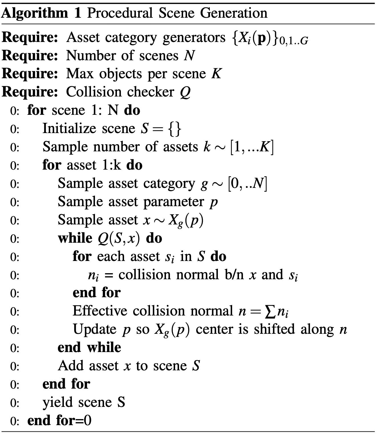
- Setup: You want to generate total scenes. For a single scene , you decide it will hold total objects.
- Initial placement: Pick an object (e.g., microwave) and drop it into the scene based on its starting parameters
- Collision check:
while(Q, s)- check if the new object is overlapping with any existing objects in the scene- Calculating the escape route: if there's a collision, for every object touches, calculate the collision normal () → sum up all normals to get the direction of the most efficient path out of the collision pile ("effective collision normal vector)
- Shift 's position slightly along , repeat loop at (3) until the object is no longer colliding with anything → then add it to the scene and move onto the next object.
Example of scenes in the dataset:

Parametrically variable categories
- 6 parametrically variable categories - shelves, cubbies, microwaves, dishwashers, open boxes, and cabinets
- "parametrically variable" - object is a flexible template driven by a set of adjustable params (i.e., shelf =
shelf(width, height, depth, number of horizontal boards, thickness of boards))
- "parametrically variable" - object is a flexible template driven by a set of adjustable params (i.e., shelf =
- (More details into Algorithm 1, read into more later.)
Objaverse assets for everyday objects
- Augment dataset with wide variety of objects that the neural planner is likely to observe during deployment (comic books, jars, record players, caps, ...)
- Sample these Objaverse assets in the "task-relevant sampling location of the programmatic asset(s) in the scene" - e.g. between shelf rungs, inside cubbies, within cabinets (there is some predefined set of "places where random objects might be found," the algorithm randomly samples from this to place Objaverse assets)
Complex scene generation
- ❓ How to combine the procedurally generated assets + Objaverse assets into a complex scene?
- Naive approach: rejection-sampling based on collision, i.e. something like -
- Pick a random 3D coordinate in the room
- Place the object there and check for collisions
- If the object collides with anything, delete it
- Repeat step (1) and pick a totally new random coordinate until you find an empty spot
- ⚠️ ^ problem with this approach: will take a very long time if the goal is to get a complex, realistic scene (e.g. a messy kitchen with appliances, utensils, open cabinets...) - if the room is 80% full, the probability of randomly guessing a safe spot is very low.
- because it's so hard to place objects in a crowded scene, this method naturally biases the training data toward sparse, simple scenes - not good!
- Their approach: effective collision normal vector
- Naive approach: rejection-sampling based on collision, i.e. something like -
Motion planning experts
AIT* + smoothing using cubic spline interpolation + enforced velocity and acceleration limits.
- 📍 Read into more later
Architecture for creating a generalist neural policies
Model input
- Represent scene using point-clouds grounded in the base frame of the robot ()
- Overlay the scene point-cloud with current robot mesh (generated from joint angles ) and target robot mesh (joint angles ):
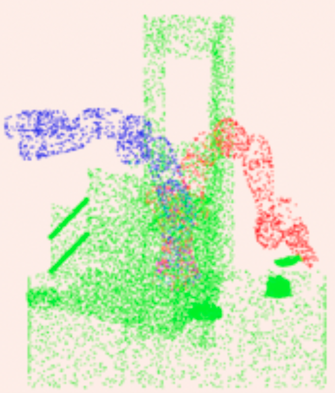
- Overlay the scene point-cloud with current robot mesh (generated from joint angles ) and target robot mesh (joint angles ):
- Current joint angles
- Target joint angles
Model architecture
- 🔑 They formulate the problem of learning motion planning as a "multi-modal sequential control problem"
- multi-modal inputs: both high-dim spatial vision () and low-dim kinematics (, )
- handle by using separate encoders -
- encode point-clouds using PointNet++
- they follow design decisions from MπNets regarding point-cloud observations (segment robot, obstacle, target point cloud before passing to PointNet++)
- encode and using MLPs
- encode point-clouds using PointNet++
- handle by using separate encoders -
- sequential: motion planning is not a one-shot prediction; it is a trajectory of states and actions over time - the model should have temporal context
- handle by using LSTM policy
- 🔖 they find that LSTMs have comparable performance to transformers on their datasets (Appendix)
- handle by using LSTM policy
- 📍 at each time-step, they concat the embeddings of each of the inputs together → pass to LSTM → GMM → output
- multi-modal outputs: there are multiple literal modes that the model needs to be capable of representing - i.e. for the same task (scene + target), the expert planner might generate one path that goes left and another path that goes right → the model needs to learn distinct "modes" of behavior
- handle by feeding output of LSTM to a Gaussian mixture model (GMM)
- 🔖 NeuralMP predicts a GMM distribution over , which are used to compute the next target joint waypoint during deployment:
- multi-modal inputs: both high-dim spatial vision () and low-dim kinematics (, )
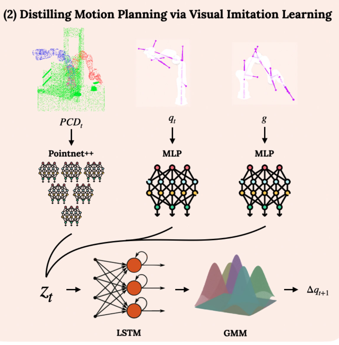
Essentially ^: the LSTM is the brain and the GMM is the format of the answer (mixture density network!)
LSTM + GMM details
- 💡 Intuition: LSTM outputs the parameters of a probability distribution (GMM)
- GMM is not a neural network layer - it's just a statistical equation!
- Concrete implementation in NeuralMP:
- Numbers:
- LSTM hidden state size: 1024
- Action space : 7 (7 dof Panda arm predicting delta joint angles )
- GMM modes : 5 (the network is allowed to suggest up to 5 different distinct movement paths)
- To define a GMM with 5 modes for a 7D action, the LSTM needs to output:
- Mixture weights : which of the 5 paths is most likely? (requires 5 numbers)
- Means : what is the exact 7-joint movement for each of the 5 paths? (requires 5x7 = 35 numbers)
- Standard deviations : how much uncertainty is there around each of those 5 paths? (requires 5x7 = 35 numbers)
- ^ Total outputs needed: numbers
- Step-by-step walkthrough model forward pass, starting from LSTM output:
- LSTM outputs a vector of size
[1024] - Linear layer -
[1024]→[75] - Split - the model slices
[75]intoweights_raw,means_raw,stddevs_raw - Activations -
weights_rawpassed through softmax fn so that it sums to 1 (probabilities can't be negative),means_rawis fine,stddevs_rawpassed through exp/softplus to ensure they are strictly positive numbers - The model now has output a fully formed GMM!
- To move the robot - sample from this distribution ^
- Select a mode by sampling from the GMM's mixture weights
- Sample from the selected mode's
meanandstddevvector (Gaussian)! → this final sampled action is
- LSTM outputs a vector of size
- Numbers:
Loss functions
NeuralMP uses GMM negative log-likelihood as their training loss, and finds that it outperforms the loss functions employed in MπNets, diffusion (EDMP), & action-chunking (ACT).
- Loss types that they test:
- GMM log-likelihood - the PDF of the true action given the predicted GMM params (from the model output) is: where the multi-dim. diagonal Gaussian profile is calculated as: To train the network, we minimize NLL: (Core logic of NLL loss: minimize NLL → maximize log-likelihood → maximize likelihood → maximize , where = expert behavior)
- 💡 GMM NLL is safe from mode averaging because: [work through the math in detail later] through the chain rule, the gradient of wrt. the mean of a specific component reveals a term called the posterior responsibility ():
- Think of GMM as a committee of experts. is called "responsibility" because it measures how much expert is "responsible" for this data point (and thereby should be gradient updated by the loss incurred due to this data point)
- If an expert's responsibility is 0.99, they get 99% of the gradient update - they move to match
- This is how GMM avoids mode averaging! It allows different experts to refine to different modes.
- "posterior" comes from the fact that the equation for is effectively Bayes' theorem - it measures: "what is the probability that expert generated this action, given the action we just saw?" The gradient for the mean vector simplifies down to: So, if the expert's action matches left (), the Gaussian component representing the left path will have a high probability density, making its responsibility . It receives a strong gradient update to align its mean perfectly with the expert.
- ^ simultaneously, the component representing the right path is "far away" (i.e. the distance between the target and this component's mean is large enough that the responsibility of this component becomes 0) - so it doesn't get gradient updated by (as desired!)
- 🔑 GMM NLL bypasses the mode averaging problem!
- Think of GMM as a committee of experts. is called "responsibility" because it measures how much expert is "responsible" for this data point (and thereby should be gradient updated by the loss incurred due to this data point)
- 💡 GMM NLL is safe from mode averaging because: [work through the math in detail later] through the chain rule, the gradient of wrt. the mean of a specific component reveals a term called the posterior responsibility ():
- L2 loss - squared Euclidean distance between the network's single predicted action vector and the expert's true action vector
- ⚠️ L2 suffers on multi-modal data because: let's take a look at the derivative of the loss wrt. the network's prediction - During training, the optimizer updates the weights to set the expected gradient to 0. If the dataset contains an identical environment context where the expert goes left () half the time and right () the other half, the expected gradient becomes: Minimizing L2 loss is mathematically equivalent to forcing the network to output the conditional mean , and on multi-modal distributions, this results in mode averaging - yikes!
- L1 loss - absolute linear distance between the prediction and the target The derivative of the absolute value function is the sign function, so:Minimizing L1 loss (setting expected gradient to 0) forces the network to output the conditional median of the data distribution, which is the point at which and (where is the random variable that might = left/right/...) → also mode averaging!
- PointMatch loss (MπNets) - this loss optimizes directly in Cartesian space (not in joint-space), and takes a combined L2 + L1 loss form in the MπNets (but the NeuralMP formula below focuses on the L2 component, [theoretically the analysis shouldn't change much for the original L2 + L1 loss? but have yet to verify this]):
- ⚠️ Problem: FK is many-to-one when the robot has free DoF's, which causes rotational blind spots (e.g., if a robot's spherical wrist joint rotates by 180˚, the keypoints on a symmetric parallel-jaw gripper end up in nearly identical spatial locations, causing despite the massive orientational error).
- [TODO FILL IN WHAT WAS WRONG WITH THIS] - im also confused as to why pointmatch said that having the loss in task-space rather than C-space is good (citing this as an explicit design decision) while NeuralMP appears to be arguing the opposite ??
- GMM log-likelihood - the PDF of the true action given the predicted GMM params (from the model output) is: where the multi-dim. diagonal Gaussian profile is calculated as: To train the network, we minimize NLL: (Core logic of NLL loss: minimize NLL → maximize log-likelihood → maximize likelihood → maximize , where = expert behavior)
- Their results:
- They trained four identical versions of NeuralMP using the same 100K traj dataset:
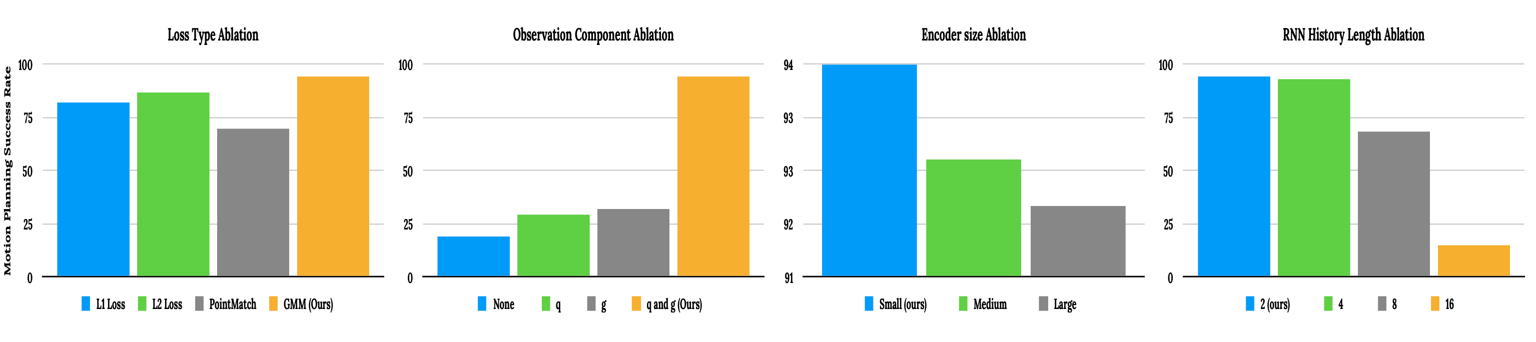
- Their model + GMM loss: 94% (motion planning success rate - end pose accuracy + collision-free)
- Their model + L2 loss: 87%
- Their model + L1 loss: 82%
- Their model + PointMatch loss: 70%
- They trained four identical versions of NeuralMP using the same 100K traj dataset:
RNN history length
[Read into later!]
Deploying neural motion planners
Test-time optimization
TL;DR: NeuralMP combines the learned policy with a "simple light-weight optimization procedure at inference time" := simulate 100 trajectories in robot brain, pick the one that is safest (with robot farthest away from obstacles in environment throughout traj.)
- 🔖 Assumptions of this optimization procedure:
- Obstacles do not move
- Controller can accurately reach the target waypoints
Given world state ( is the environment state), the predicted world state is where is the policy prediction.
- 🔑 Test-time optimization procedure: Sample trajectories from the policy using the initial scene point-cloud, estimate the number of scene points that intersect the robot, choose the traj. with least robot-scene intersection in the env. using the robot SDF:
- 💡 Objective at test time: where := distribution of trajectories under policy , := th point of the obstacle point-cloud (max points), := SDF of the robot at the current joint angles, := distance safety margin.
- ^ i.e. generate trajectories, compute objective for each traj., select traj. with minimal objective val.
NeuralMP selects the traj. with minimal objective value ^ across 100 generated trajectories.
Note: In the closed-loop case, NeuralMP takes new point-cloud snapshots + reruns the single-step optimization (collision SDF sorting) at each time step, but the open-loop deployment relies on a static scene.
Sim2real & deployment
- 4 extrinsically calibrated Intel RealSense cameras positioned at the table's corners
- Segmented point-cloud is produced via:
- Generate point-cloud of the scene using 4 cameras
- Segment out the partial robot cloud using a mesh-based repr. of the robot to exclude robot points from the generated scene point-cloud in step (1)
- Generate the current robot + target robot point clouds using FK on the robot mesh repr. and paste into the scene.
- Robot SDF computed between scene point-cloud and spherical representation of robot
- Traditional SDF method (CHOMP, TrajOpt) - look at static env, compute voxel SDF grid → divide the room into tiny 3D cubes and calculate how far each cube is from the nearest obstacle
- Once this ^ heavy calculation is done, the moving robot queries this static grid (assuming environment is largely static)
- Robot SDF (Neural MP's method) - for a sphere with center and radius , the SDF distance to any env. point is: To check for collisions at timestep :
- Use FK to find the center coordinates of the 56 robot spheres
- For all points in the obstacle cloud, compute
- ^ If any , we have a collision ( would be the exact boundary, they probably have slightly larger than 0 for a safety margin)
- Traditional SDF method (CHOMP, TrajOpt) - look at static env, compute voxel SDF grid → divide the room into tiny 3D cubes and calculate how far each cube is from the nearest obstacle
Experimental setup
4 types of start () and goal () angle pairs:
- free space to free space
- free space to tight space
- tight space to free space
- tight space to tight space
4 eval environments: 5. Bins - moving in-between, around, inside 6. Shelf - moving in-between and around the rungs 7. Articulated - moving inside and within cubbies, drawers, doors 8. In-hand - moving between rungs of a shelf while holding different objects
- 🔖 All eval is done using open loop planning, although NeuralMP is capable of closed loop planning in the same sense that MπNets is capable of closed loop planning
- They use the same definitions of success as MπNets
- They compare with:
- Sampling-based motion planning
- AIT*
- Curobo
- Neural motion planning
- SOTA - MπNets
- Sampling-based motion planning
Experimental results
- Free hand motion planning:
- Neural MP (with test-time optimization) does best! 95.83% success rate
- without test-time opt - Neural MP gets 66.67% success rate
- ⚠️ MπNets performs poorly across the board - authors theorize that:
- MπNets is only trained on data in which the expert goes from tight spaces to tight spaces - fails to generalize well to start/goal configs in free space
- End-effector point matching loss in MπNets fails to distinguish between 0 and 180˚ rotations of the EE - so the network has not learned how to match ambiguous target end-effector poses
- though even after changing the success metric for Mπnets to count 180˚ flipped EE poses as success as well, the avg success rate of MπNets only improves from 16.67% to 29.17%
- ⚠️ Failure cases for AIT and Curobo → tight spaces where vision-based collision checking is inaccurate / when probability of sampling/optimizing for a valid path is low
- Neural MP (with test-time optimization) does best! 95.83% success rate
- In hand motion planning:
- Neural MP, training with Objaverse data & w/ test-time opt.: 88% success
- Neural MP, training w/o Objaverse data & w/ test-time opt.: 44% success
- Neural MP, training w/ Objaverse data & w/o test-time opt.: 31% success
- 🔖 Neural MP performs well on in-distribution objects but struggles on OOD objects
Key conclusions:
- Test-time opt. is important for minimizing collisions → increasing success rate
- Training on Objaverse data is important - models trained only on cuboid-based parametric assets fail to generalize to the complexity of the real world (43.75%), while those trained on Objaverse perform well (81.25%) [can't actually clearly trace these numbers to a specific table but this is what the main text says]
- 🔖 NeuralMP outperforms EDMP & MπNets on the MπNets dataset in simulation
- 🔑 Authors theorize this is due to:
- use of sequence modeling
- ability of the GMM to fit multimodal data
- test-time opt. to prune out collisions
- 🔑 Authors theorize this is due to:
- Authors find that performance scales with more data (1K traj not enough, 1M traj. doing pretty well)
Dynamic motion planning
- To handle dynamic obstacles - run NeuralMP closed loop and perform single-step test-time opt.
- NeuralMP performs 53% better than MπNets.
Ablations
Evaluates performance on held out scenes for each ablation.
- Training objective: (i.e. loss function)
- GMM > L2 > L1 > PointMatch
- Model input: (they call this "observation composition")
- Using and vectors is crucial for performance
- vs. MπNets only uses
- Using and vectors is crucial for performance
Discussion & limitations
- 2.5x-20x faster, >20% motion planning success rate compared to AIT*
Future improvements
- NeuralMP model is susceptible to point-cloud quality
- can potentially improve 3D representations via implicit models - e.g. NeRFs
- NeuralMP model does not handle tight spaces well
- could potentially fine-tune base policy w/ RL
- NeuralMP model is slower than simply running the policy directly due to test-time opt.
- can be addressed by leveraging learned collision checking - https://arxiv.org/pdf/2304.09302, https://arxiv.org/pdf/2011.10726
My key takeaways
- Can we also use GMM as the final model output form + GMM log-likelihood?
- Our output is also multimodal - elbow up vs. down, base positions, ...
- Could have drifting model output , and then sample from the GMM, i.e. where is the final model output
- LSTM with context window of current robot config - vs. sampling-time guidance to push it to be close to the current robot config?
- What loss should we do / how does drifting loss hold up to preventing (or potentially causing) mode averaging?
- Can we use GMM NLL too to prevent mode averaging?
- "test-time optimization" is basically a "think before you move" filter for the robot - generate 100 possible trajectories, pick the safest one ("safe" defined via metric computed using robot SDF)
- We can do this for model_ik by sampling 100 seeds → refine → pick the one with greatest robot SDF<->environment at this time frame - i.e. where is the total number of points in the obstacle point cloud.
- ❓ Do we need to feed the model negative and positive examples of collision? [Design decision to make]
- NeuralMP and MπNets seem to both only train on clean data (so the model never sees collisions) - but ViIK trains on both & has the model output an
is_collidingflag along with output so that it learns the boundaries of collisions - ^ could test both methods?
- NeuralMP and MπNets seem to both only train on clean data (so the model never sees collisions) - but ViIK trains on both & has the model output an
- Compute robot SDF using NeuralMP's method to be faster (0.01-0.02s per query) [lacks precision for tight spaces but seems largely OK]
- SDF between the scene point-cloud and the spherical representation of the robot
Footnotes
Pf: Minimizing L2 loss pushes the network to output the conditional mean
Setup: Let's call the input to the neural network and its output prediction . The network's goal is to choose a prediction that minimizes the Expected L2 loss across all possible true answers. Because the training dataset might have multiple different valid answers for this exact same scene , the true target that we want the model to learn is not a single number, but a random variable drawn from some probability distribution .
- Define the expected loss: The expected L2 loss (aka. "risk") for our prediction , given the input , is written as:
- Expand the square:
- Apply linearity of expectation:
- Find the minimum via calculus: to find the value of that minimizes , we take the derivative of and set it to 0. is a constant relative to , so we end up with:
- Therefore: . We can check the 2nd derivative to ensure this is a minimum and not a maximum: Because , the function is convex, meaning we have found the global minimum.
^ This math proves that if you train a network with L2 loss until it perfectly converges, its prediction will mathematically equal - the conditional mean (average of all possible true targets for that input).